Graphs A R Hadaegh Dr Ahmad R Hadaegh

Graphs A. R. Hadaegh Dr. Ahmad R. Hadaegh California State University San Marcos (CSUSM) Page 1

• One limitation of the trees is that the trees are hierarchal in nature. They only represent relations of hierarchal types such as relations between parents and child • A generalization of tree, called GRAPH, is a data structure in which these limitations are lifted • A graph is a collection of vertices (nodes) and connection between them called edges • A simple graph G= (V, E) consists of a nonempty set of V of vertices and possibly empty set E of edges where each edge is a connection between two vertices • The number of vertices and edges of a graph are represented as |V| and |E|, respectively. A. R. Hadaegh Dr. Ahmad R. Hadaegh California State University San Marcos (CSUSM) Page 2

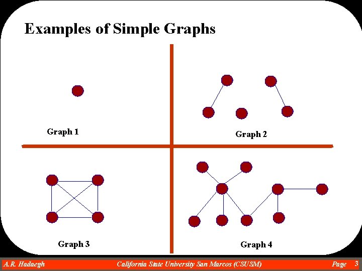
Examples of Simple Graphs Graph 1 Graph 3 A. R. Hadaegh Dr. Ahmad R. Hadaegh Graph 2 Graph 4 California State University San Marcos (CSUSM) Page 3

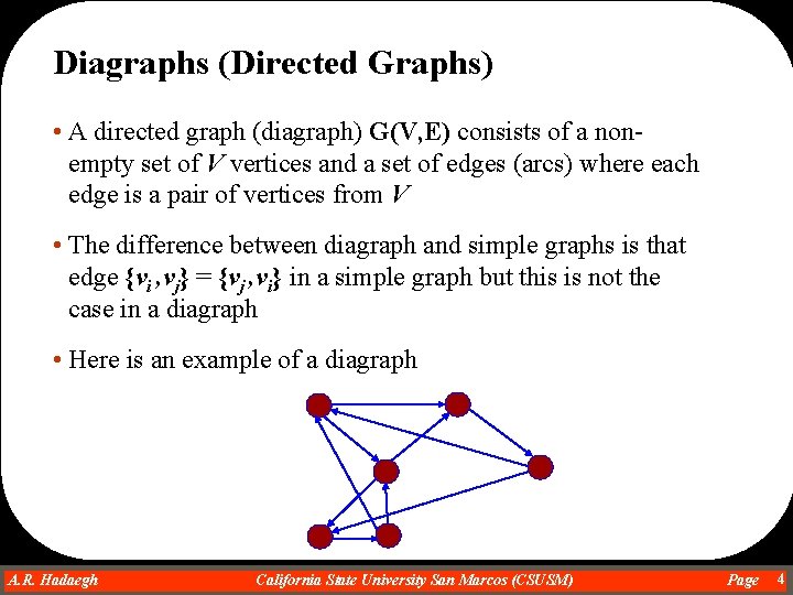
Diagraphs (Directed Graphs) • A directed graph (diagraph) G(V, E) consists of a nonempty set of V vertices and a set of edges (arcs) where each edge is a pair of vertices from V • The difference between diagraph and simple graphs is that edge {vi , vj} = {vj , vi} in a simple graph but this is not the case in a diagraph • Here is an example of a diagraph A. R. Hadaegh Dr. Ahmad R. Hadaegh California State University San Marcos (CSUSM) Page 4

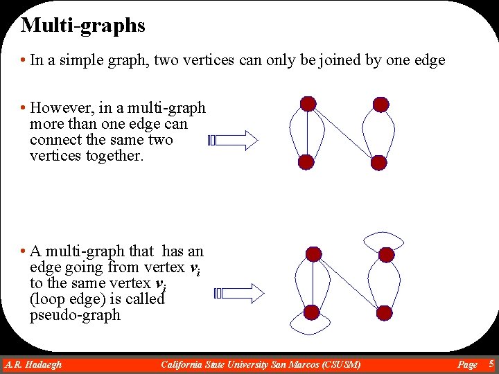
Multi-graphs • In a simple graph, two vertices can only be joined by one edge • However, in a multi-graph more than one edge can connect the same two vertices together. • A multi-graph that has an edge going from vertex vi to the same vertex vi (loop edge) is called pseudo-graph A. R. Hadaegh Dr. Ahmad R. Hadaegh California State University San Marcos (CSUSM) Page 5

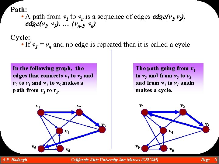
Path: • A path from v 1 to vn is a sequence of edges edge(v 1, v 2), edge(v 2, v 3), … (vn-1, vn) Cycle: • If v 1 = vn and no edge is repeated then it is called a cycle In the following graph, the edges that connects v 1 to v 2 and v 2 to v 3 and v 3 to v 5 makes a path from v 1 to v 5. v 1 A. R. Hadaegh Dr. Ahmad R. Hadaegh v 1 v 2 v 4 v 5 The path going from v 1 to v 2 and from v 2 to v 3 and from v 3 to v 1 again makes a cycle. v 6 v 3 v 2 v 4 v 5 California State University San Marcos (CSUSM) v 3 v 6 Page 6

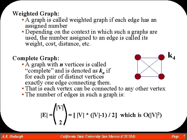
Weighted Graph: • A graph is called weighted graph if each edge has an assigned number • Depending on the context in which such a graphs are used, the number assigned to an edge is called its weight, cost, distance, etc. Complete Graph: • A graph with n vertices is called “complete” and is denoted as kn if for each pair of distinct vertices exactly one edge connecting them. • That is each vertex can be connected to any other vertex • The number of edges in such a graph is: k 4 |V| |E| = = [ |V| * (|V|-1) / 2] which is O(|V|2) 2 A. R. Hadaegh Dr. Ahmad R. Hadaegh California State University San Marcos (CSUSM) Page 7

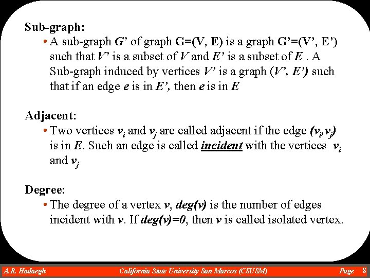
Sub-graph: • A sub-graph G’ of graph G=(V, E) is a graph G’=(V’, E’) such that V’ is a subset of V and E’ is a subset of E. A Sub-graph induced by vertices V’ is a graph (V’, E’) such that if an edge e is in E’, then e is in E Adjacent: • Two vertices vi and vj are called adjacent if the edge (vi, vj) is in E. Such an edge is called incident with the vertices vi and vj Degree: • The degree of a vertex v, deg(v) is the number of edges incident with v. If deg(v)=0, then v is called isolated vertex. A. R. Hadaegh Dr. Ahmad R. Hadaegh California State University San Marcos (CSUSM) Page 8

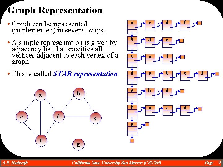
Graph Representation • Graph can be represented (implemented) in several ways. a c d • A simple representation is given by adjacency list that specifies all vertices adjacent to each vertex of a graph b d e c a f • This is called STAR representation d a b e b d f a c b a d c f e f d e g f A. R. Hadaegh Dr. Ahmad R. Hadaegh g California State University San Marcos (CSUSM) Page 9

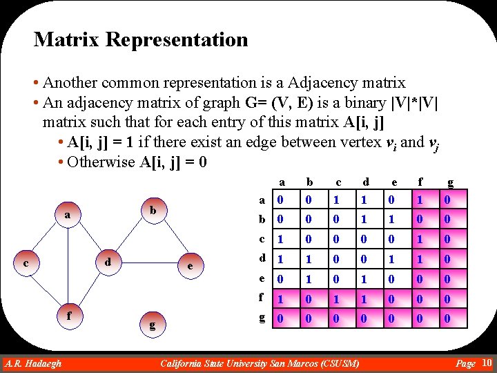
Matrix Representation • Another common representation is a Adjacency matrix • An adjacency matrix of graph G= (V, E) is a binary |V|*|V| matrix such that for each entry of this matrix A[i, j] • A[i, j] = 1 if there exist an edge between vertex vi and vj • Otherwise A[i, j] = 0 d c f A. R. Hadaegh Dr. Ahmad R. Hadaegh e g b 0 c 1 d 1 e 0 f 1 g 0 b 0 0 0 1 1 0 0 c 1 0 0 1 0 d 1 e 0 1 0 0 1 1 0 1 0 0 0 f 1 0 1 1 0 0 0 g 0 0 0 0 a b a a 0 California State University San Marcos (CSUSM) Page 10

Comparison: • Which representation is better? • Think about searching for an edge • Think about printing all edges • Think about inserting an edge • How about inserting a vertex • How about deleting an edge A. R. Hadaegh Dr. Ahmad R. Hadaegh California State University San Marcos (CSUSM) Page 11

Graph Traversal • Two systematic method for traversal of graph are depth-first traversal and breadth-first traversal • Of course since graph may contain cycle, they have different structure compare to trees • Therefore, traversal algorithms we used for trees cannot be applied for graphs exactly the same way and they should be modified to fit the graph requirements • Further, not all graphs are connected. A graph may contain isolated trees, isolated graphs or isolated vertices. • In a connected graph, we can find a path between any two vertices in the graph but this is not the case for unconnected graphs A. R. Hadaegh Dr. Ahmad R. Hadaegh California State University San Marcos (CSUSM) Page 12

Depth-First Traversal Using Recursion • A vertex v is visited once then each adjacent vertex to v is visited and so on • If vertex v has no adjacent vertex or all of its adjacent vertices have already been visited, we backtrack to the predecessor of v • The traversal is finished if this visiting and backtracking process leads to the first vertex where the traversal started • Finally, if there is still some unvisited vertex in the graph, the traversal continues for one of the unvisited vertices A. R. Hadaegh Dr. Ahmad R. Hadaegh California State University San Marcos (CSUSM) Page 13

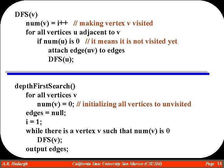
DFS(v) num(v) = i++ // making vertex v visited for all vertices u adjacent to v if num(u) is 0 // it means it is not visited yet attach edge(uv) to edges DFS(u); depth. First. Search() for all vertices v num(v) = 0; // initializing all vertices to unvisited edges = null; i = 1; while there is a vertex v such that num(v) is 0 DFS(v); output edges; A. R. Hadaegh Dr. Ahmad R. Hadaegh California State University San Marcos (CSUSM) Page 14

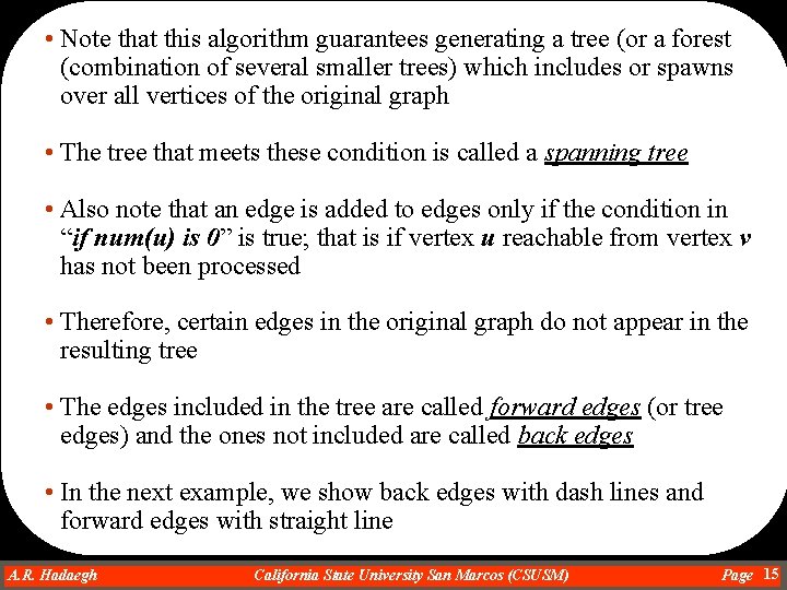
• Note that this algorithm guarantees generating a tree (or a forest (combination of several smaller trees) which includes or spawns over all vertices of the original graph • The tree that meets these condition is called a spanning tree • Also note that an edge is added to edges only if the condition in “if num(u) is 0” is true; that is if vertex u reachable from vertex v has not been processed • Therefore, certain edges in the original graph do not appear in the resulting tree • The edges included in the tree are called forward edges (or tree edges) and the ones not included are called back edges • In the next example, we show back edges with dash lines and forward edges with straight line A. R. Hadaegh Dr. Ahmad R. Hadaegh California State University San Marcos (CSUSM) Page 15

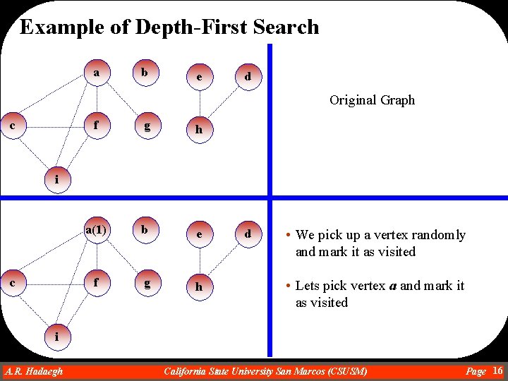
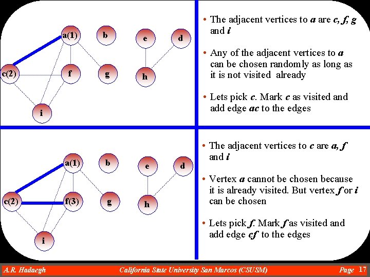
Example of Depth-First Search a b e d Original Graph c f g h a(1) b e f g h i c d • We pick up a vertex randomly and mark it as visited • Lets pick vertex a and mark it as visited i A. R. Hadaegh Dr. Ahmad R. Hadaegh California State University San Marcos (CSUSM) Page 16

a(1) c(2) f b g e d • Any of the adjacent vertices to a can be chosen randomly as long as it is not visited already h • Lets pick c. Mark c as visited and add edge ac to the edges i a(1) c(2) • The adjacent vertices to a are c, f, g and i f(3) i A. R. Hadaegh Dr. Ahmad R. Hadaegh b g e h d • The adjacent vertices to c are a, f and i • Vertex a cannot be chosen because it is already visited. But vertex f or i can be chosen • Lets pick f. Mark f as visited and add edge cf to the edges California State University San Marcos (CSUSM) Page 17

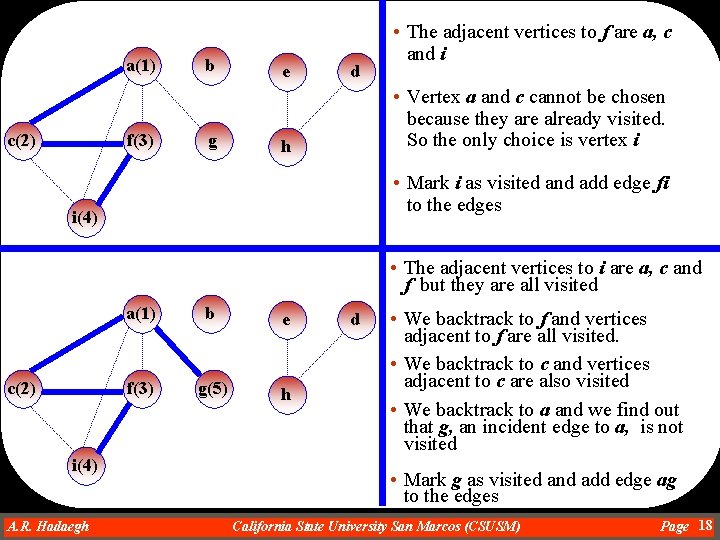
a(1) c(2) f(3) b g e d • The adjacent vertices to f are a, c and i • Vertex a and c cannot be chosen because they are already visited. So the only choice is vertex i h • Mark i as visited and add edge fi to the edges i(4) • The adjacent vertices to i are a, c and f but they are all visited c(2) a(1) b e f(3) g(5) h i(4) A. R. Hadaegh Dr. Ahmad R. Hadaegh d • We backtrack to f and vertices adjacent to f are all visited. • We backtrack to c and vertices adjacent to c are also visited • We backtrack to a and we find out that g, an incident edge to a, is not visited • Mark g as visited and add edge ag to the edges California State University San Marcos (CSUSM) Page 18

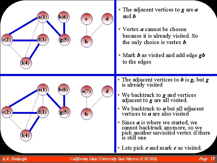
a(1) c(2) f(3) b(6) g(5) e d • Vertex a cannot be chosen because it is already visited. So the only choice is vertex b h • Mark b as visited and add edge gb to the edges i(4) c(2) • The adjacent vertices to g are a and b • The adjacent vertices to b is g, but g is already visited a(1) b(6) e(7) f(3) g(5) h i(4) d • We backtrack to g and vertices adjacent to g are all visited. • We backtrack to a but all adjacent vertices to a are also visited • Since a is where we started, we cannot backtrack anymore, so we pick another unvisited vertex if there is still one • Lets pick e and mark e as visited. A. R. Hadaegh Dr. Ahmad R. Hadaegh California State University San Marcos (CSUSM) Page 19

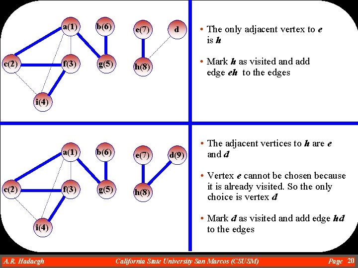
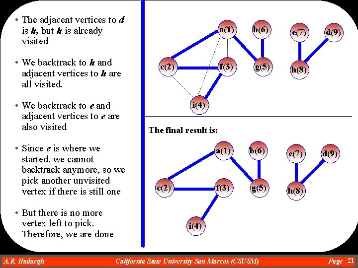
c(2) a(1) b(6) e(7) f(3) g(5) h(8) d • The only adjacent vertex to e is h • Mark h as visited and add edge eh to the edges i(4) a(1) c(2) f(3) i(4) A. R. Hadaegh Dr. Ahmad R. Hadaegh b(6) g(5) e(7) h(8) d(9) • The adjacent vertices to h are e and d • Vertex e cannot be chosen because it is already visited. So the only choice is vertex d • Mark d as visited and add edge hd to the edges California State University San Marcos (CSUSM) Page 20

• The adjacent vertices to d is h, but h is already visited • We backtrack to h and adjacent vertices to h are all visited. • We backtrack to e and adjacent vertices to e are also visited • Since e is where we started, we cannot backtrack anymore, so we pick another unvisited vertex if there is still one • But there is no more vertex left to pick. Therefore, we are done A. R. Hadaegh Dr. Ahmad R. Hadaegh c(2) a(1) b(6) e(7) f(3) g(5) h(8) d(9) i(4) The final result is: c(2) a(1) b(6) e(7) f(3) g(5) h(8) d(9) i(4) California State University San Marcos (CSUSM) Page 21

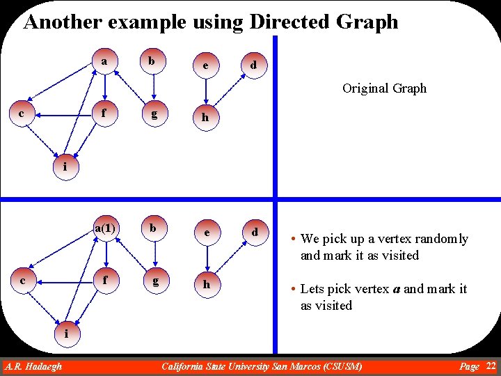
Another example using Directed Graph a b e d Original Graph c f g h a(1) b e f g h i c d • We pick up a vertex randomly and mark it as visited • Lets pick vertex a and mark it as visited i A. R. Hadaegh Dr. Ahmad R. Hadaegh California State University San Marcos (CSUSM) Page 22

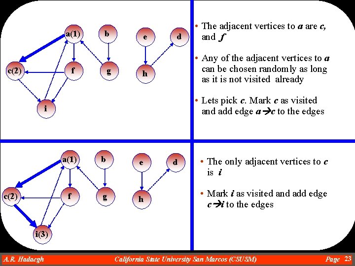
a(1) c(2) b f g e d • Any of the adjacent vertices to a can be chosen randomly as long as it is not visited already h • Lets pick c. Mark c as visited and add edge a c to the edges i c(2) • The adjacent vertices to a are c, and f a(1) b e f g h d • The only adjacent vertices to c is i • Mark i as visited and add edge c i to the edges i(3) A. R. Hadaegh Dr. Ahmad R. Hadaegh California State University San Marcos (CSUSM) Page 23

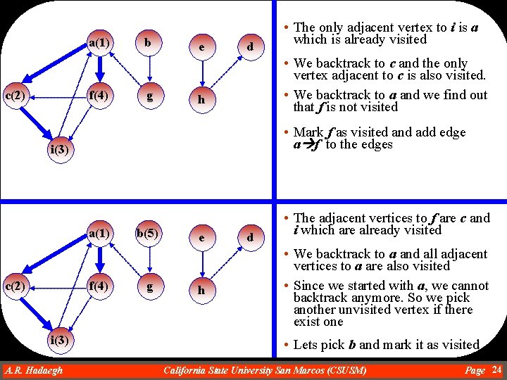
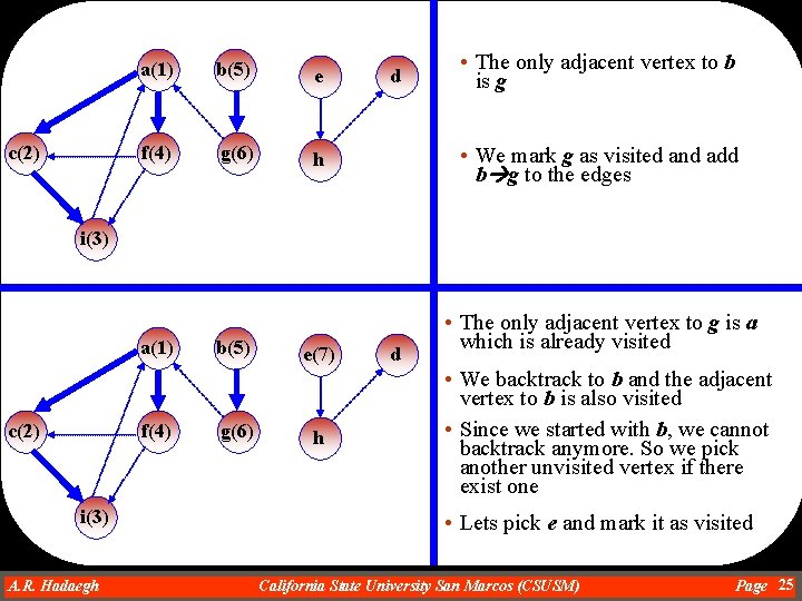
a(1) c(2) f(4) b g e d • We backtrack to c and the only vertex adjacent to c is also visited. • We backtrack to a and we find out that f is not visited h • Mark f as visited and add edge a f to the edges i(3) a(1) c(2) • The only adjacent vertex to i is a which is already visited f(4) i(3) A. R. Hadaegh Dr. Ahmad R. Hadaegh b(5) g e h d • The adjacent vertices to f are c and i which are already visited • We backtrack to a and all adjacent vertices to a are also visited • Since we started with a, we cannot backtrack anymore. So we pick another unvisited vertex if there exist one • Lets pick b and mark it as visited California State University San Marcos (CSUSM) Page 24

c(2) a(1) b(5) e f(4) g(6) h d • The only adjacent vertex to b is g • We mark g as visited and add b g to the edges i(3) a(1) c(2) f(4) i(3) A. R. Hadaegh Dr. Ahmad R. Hadaegh b(5) g(6) e(7) h d • The only adjacent vertex to g is a which is already visited • We backtrack to b and the adjacent vertex to b is also visited • Since we started with b, we cannot backtrack anymore. So we pick another unvisited vertex if there exist one • Lets pick e and mark it as visited California State University San Marcos (CSUSM) Page 25

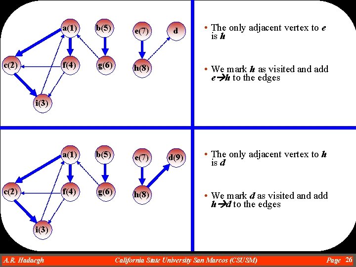
c(2) a(1) b(5) e(7) f(4) g(6) h(8) d • The only adjacent vertex to e is h • We mark h as visited and add e h to the edges i(3) c(2) d(9) • The only adjacent vertex to h is d • We mark d as visited and add h d to the edges i(3) A. R. Hadaegh Dr. Ahmad R. Hadaegh California State University San Marcos (CSUSM) Page 26

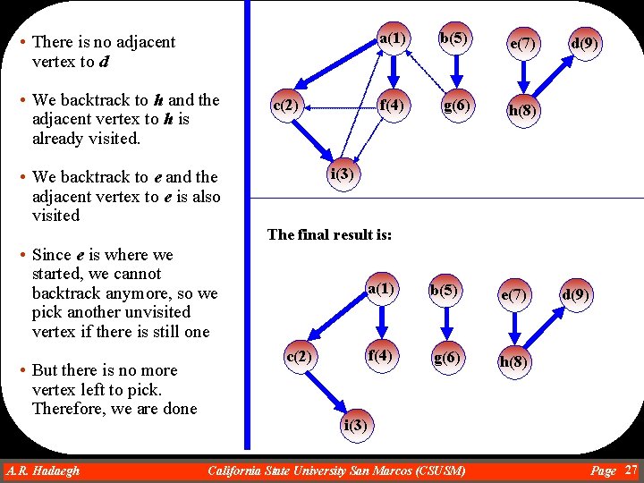
• There is no adjacent vertex to d • We backtrack to h and the adjacent vertex to h is already visited. c(2) a(1) b(5) e(7) f(4) g(6) h(8) d(9) i(3) • We backtrack to e and the adjacent vertex to e is also visited The final result is: • Since e is where we started, we cannot backtrack anymore, so we pick another unvisited vertex if there is still one • But there is no more vertex left to pick. Therefore, we are done A. R. Hadaegh Dr. Ahmad R. Hadaegh c(2) a(1) b(5) e(7) f(4) g(6) h(8) d(9) i(3) California State University San Marcos (CSUSM) Page 27

Complexity of depth-first search • The complexity of depth. First. Search() is O(|V| + |E|) because: • Initializing num(v) for each vertex requires |V| steps • DFS(v) is called deg(v) times for each v; that is, once for each edge of v (to spawn into more calls or to finish the chain of recursive calls), hence, the total number of calls is 2|E| because each edge is adjacent to two vertices • Searching for vertices as required by the statement While there is vertex v such that num(v) is 0 • Can be assumed to require |V| steps in worse case. A. R. Hadaegh Dr. Ahmad R. Hadaegh California State University San Marcos (CSUSM) Page 28

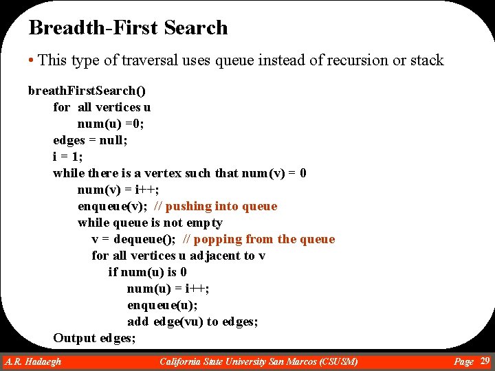
Breadth-First Search • This type of traversal uses queue instead of recursion or stack breath. First. Search() for all vertices u num(u) =0; edges = null; i = 1; while there is a vertex such that num(v) = 0 num(v) = i++; enqueue(v); // pushing into queue while queue is not empty v = dequeue(); // popping from the queue for all vertices u adjacent to v if num(u) is 0 num(u) = i++; enqueue(u); add edge(vu) to edges; Output edges; A. R. Hadaegh Dr. Ahmad R. Hadaegh California State University San Marcos (CSUSM) Page 29

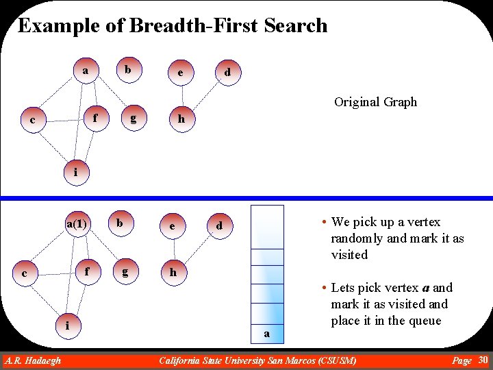
Example of Breadth-First Search b a e d Original Graph g f c h i a(1) f c i A. R. Hadaegh Dr. Ahmad R. Hadaegh b g e • We pick up a vertex randomly and mark it as visited d h a • Lets pick vertex a and mark it as visited and place it in the queue California State University San Marcos (CSUSM) Page 30

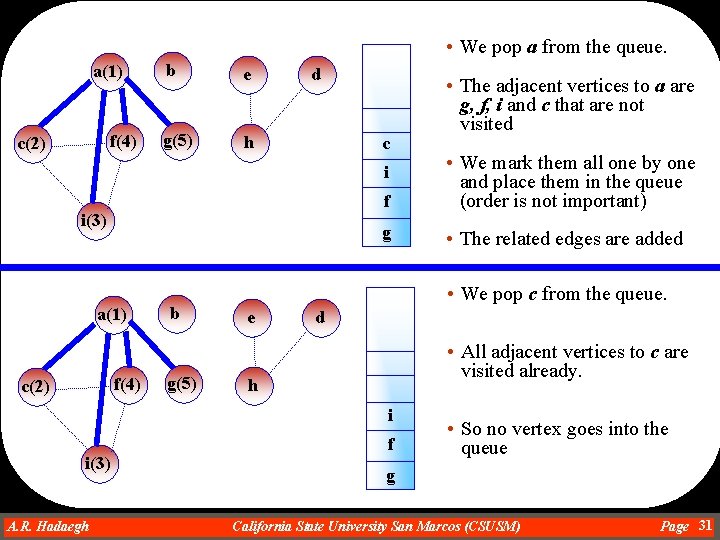
• We pop a from the queue. a(1) f(4) c(2) b e g(5) h d c f • We mark them all one by one and place them in the queue (order is not important) g • The related edges are added i i(3) a(1) f(4) c(2) b g(5) • We pop c from the queue. e d • All adjacent vertices to c are visited already. h i i(3) A. R. Hadaegh Dr. Ahmad R. Hadaegh • The adjacent vertices to a are g, f, i and c that are not visited f • So no vertex goes into the queue g California State University San Marcos (CSUSM) Page 31

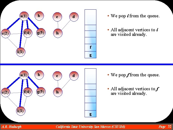
a(1) f(4) c(2) b e g(5) h • All adjacent vertices to i are visited already. f i(3) g a(1) f(4) c(2) • We pop i from the queue. d i(3) A. R. Hadaegh Dr. Ahmad R. Hadaegh b e g(5) h • We pop f from the queue. d • All adjacent vertices to f are visited already. g California State University San Marcos (CSUSM) Page 32

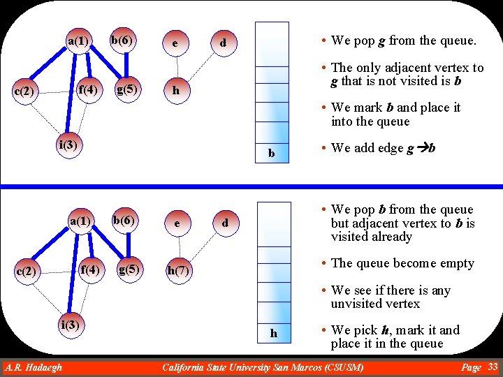
a(1) f(4) c(2) b(6) g(5) e • We pop g from the queue. d • The only adjacent vertex to g that is not visited is b h • We mark b and place it into the queue i(3) b a(1) f(4) c(2) b(6) g(5) e • We add edge g b • We pop b from the queue but adjacent vertex to b is visited already d • The queue become empty h(7) • We see if there is any unvisited vertex i(3) A. R. Hadaegh Dr. Ahmad R. Hadaegh h • We pick h, mark it and place it in the queue California State University San Marcos (CSUSM) Page 33

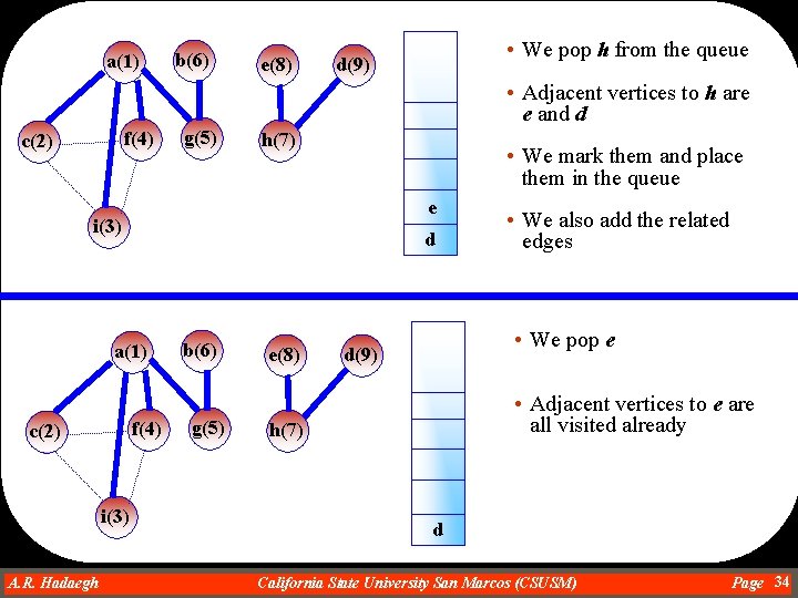
a(1) b(6) e(8) • We pop h from the queue d(9) • Adjacent vertices to h are e and d f(4) c(2) g(5) h(7) • We mark them and place them in the queue e i(3) d a(1) f(4) c(2) i(3) A. R. Hadaegh Dr. Ahmad R. Hadaegh b(6) g(5) e(8) • We also add the related edges • We pop e d(9) • Adjacent vertices to e are all visited already h(7) d California State University San Marcos (CSUSM) Page 34

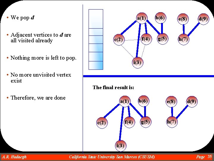
• We pop d a(1) • Adjacent vertices to d are all visited already f(4) c(2) • Nothing more is left to pop. b(6) e(8) g(5) d(9) h(7) i(3) • No more unvisited vertex exist The final result is: • Therefore, we are done a(1) f(4) c(2) b(6) g(5) e(8) d(9) h(7) i(3) A. R. Hadaegh Dr. Ahmad R. Hadaegh California State University San Marcos (CSUSM) Page 35

Finding Shortest Path • Finding the shortest path is a classical problem in graph theory • Edges of a graph are assigned certain weights representing for example, • Distance between cities • Times separating the execution of programs • Costs of transmitting data from one site to another • When determining the shortest path from vertex v to vertex u, information about distances between intermediate vertices w, has to be recorded • Several algorithms have been proposed to solve the shortest path problem A. R. Hadaegh Dr. Ahmad R. Hadaegh California State University San Marcos (CSUSM) Page 36

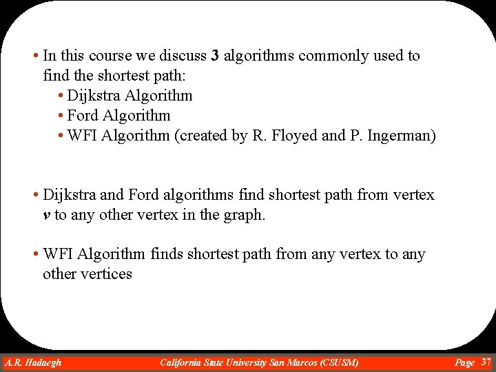
• In this course we discuss 3 algorithms commonly used to find the shortest path: • Dijkstra Algorithm • Ford Algorithm • WFI Algorithm (created by R. Floyed and P. Ingerman) • Dijkstra and Ford algorithms find shortest path from vertex v to any other vertex in the graph. • WFI Algorithm finds shortest path from any vertex to any other vertices A. R. Hadaegh Dr. Ahmad R. Hadaegh California State University San Marcos (CSUSM) Page 37

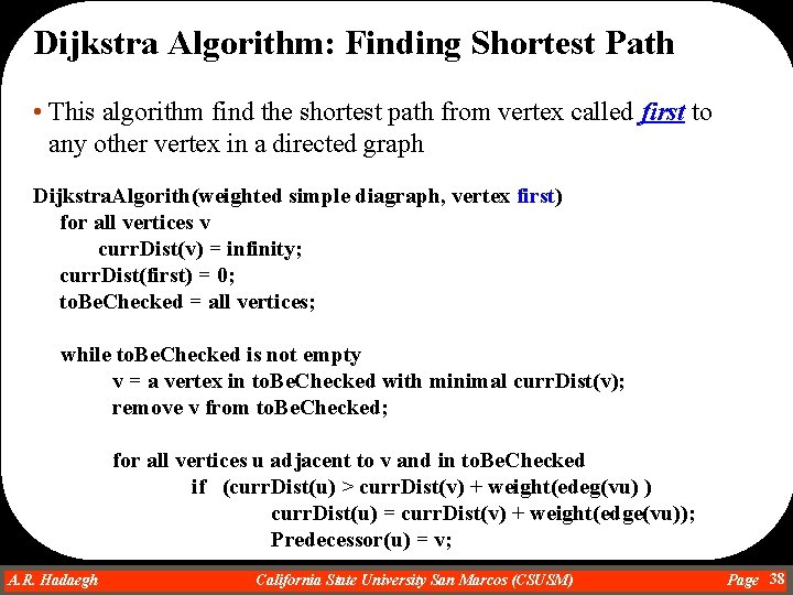
Dijkstra Algorithm: Finding Shortest Path • This algorithm find the shortest path from vertex called first to any other vertex in a directed graph Dijkstra. Algorith(weighted simple diagraph, vertex first) for all vertices v curr. Dist(v) = infinity; curr. Dist(first) = 0; to. Be. Checked = all vertices; while to. Be. Checked is not empty v = a vertex in to. Be. Checked with minimal curr. Dist(v); remove v from to. Be. Checked; for all vertices u adjacent to v and in to. Be. Checked if (curr. Dist(u) > curr. Dist(v) + weight(edeg(vu) ) curr. Dist(u) = curr. Dist(v) + weight(edge(vu)); Predecessor(u) = v; A. R. Hadaegh Dr. Ahmad R. Hadaegh California State University San Marcos (CSUSM) Page 38

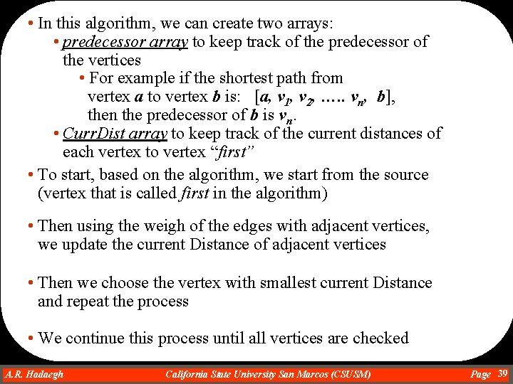
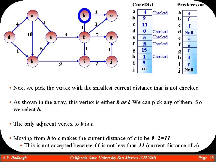
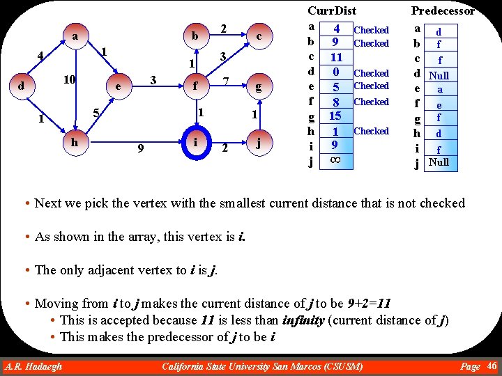
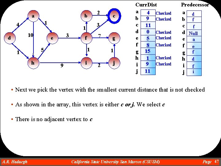
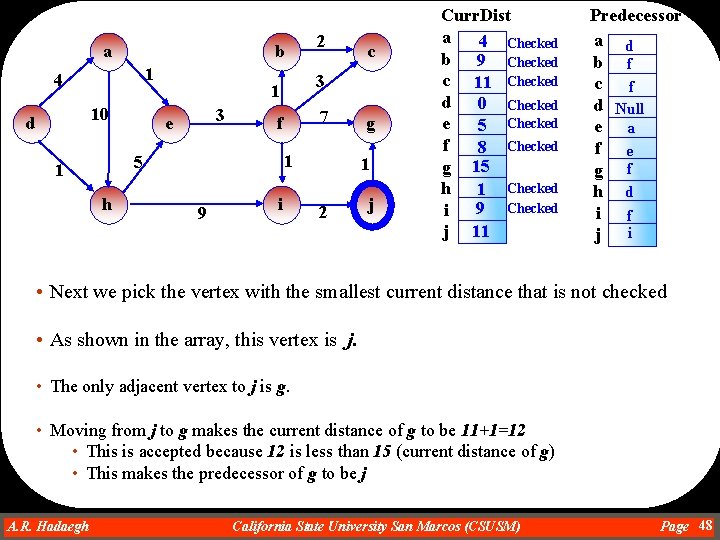
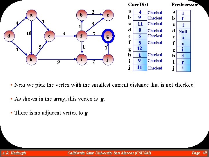
• In this algorithm, we can create two arrays: • predecessor array to keep track of the predecessor of the vertices • For example if the shortest path from vertex a to vertex b is: [a, v 1, v 2, …. . vn, b], then the predecessor of b is vn. • Curr. Dist array to keep track of the current distances of each vertex to vertex “first” • To start, based on the algorithm, we start from the source (vertex that is called first in the algorithm) • Then using the weigh of the edges with adjacent vertices, we update the current Distance of adjacent vertices • Then we choose the vertex with smallest current Distance and repeat the process • We continue this process until all vertices are checked A. R. Hadaegh Dr. Ahmad R. Hadaegh California State University San Marcos (CSUSM) Page 39

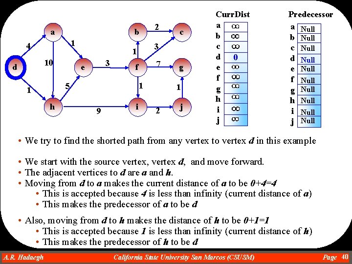
a b 1 4 10 d 3 h 7 f 1 5 1 9 i c 3 1 e 2 g 1 2 j Curr. Dist a b c d 0 e f g h i j Predecessor a Null b Null c Null d Null e Null f Null g Null h Null i Null j Null • We try to find the shorted path from any vertex to vertex d in this example • We start with the source vertex, vertex d, and move forward. • The adjacent vertices to d are a and h. • Moving from d to a makes the current distance of a to be 0+4=4 • This is accepted because 4 is less than infinity (current distance of a) • This makes the predecessor of a to be d • Also, moving from d to h makes the distance of h to be 0+1=1 • This is accepted because 1 is less than infinity (current distance of h) • This makes the predecessor of h to be d A. R. Hadaegh Dr. Ahmad R. Hadaegh California State University San Marcos (CSUSM) Page 40

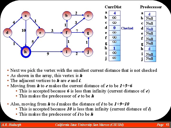
a b 1 4 10 d h 7 f 1 5 1 • • 3 9 i c 3 1 e 2 g 1 2 j Curr. Dist a 4 b c d 0 Checked e f g h 1 i j Predecessor a d b Null c Null d Null e Null f Null g Null h d i Null j Null Next we pick the vertex with the smallest current distance that is not checked As shown in the array, this vertex is h The adjacent vertices to h are e and i. Moving from h to e makes the current distance of e to be 1+5=6 • This is accepted because 6 is less than infinity (current distance of e) • This makes the predecessor of e to be h • Also, moving from h to i makes the distance of i to be 1+9=10 • This is accepted because 10 is less than infinity (current distance of i) • This makes the predecessor of i to be h A. R. Hadaegh Dr. Ahmad R. Hadaegh California State University San Marcos (CSUSM) Page 41

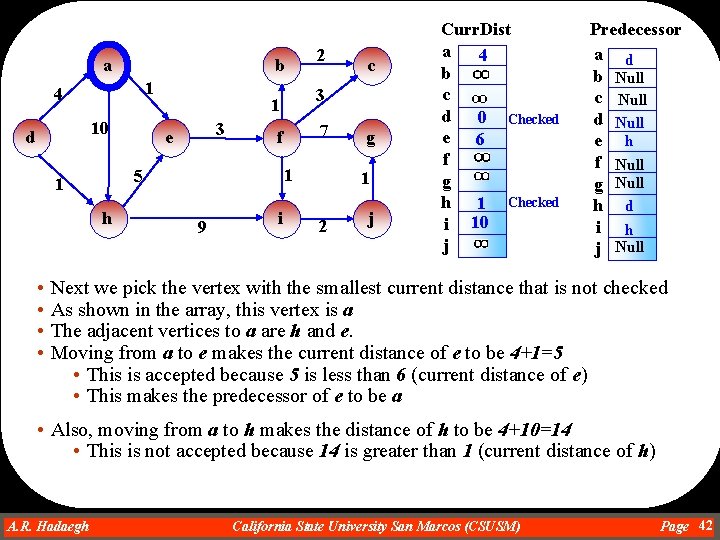
b a 1 4 10 d h 7 f 1 5 1 • • 3 9 i c 3 1 e 2 g 1 2 j Curr. Dist a 4 b c d 0 Checked e 6 f g h 1 Checked i 10 j Predecessor a d b Null c Null d Null e h f Null g Null h d i h j Null Next we pick the vertex with the smallest current distance that is not checked As shown in the array, this vertex is a The adjacent vertices to a are h and e. Moving from a to e makes the current distance of e to be 4+1=5 • This is accepted because 5 is less than 6 (current distance of e) • This makes the predecessor of e to be a • Also, moving from a to h makes the distance of h to be 4+10=14 • This is not accepted because 14 is greater than 1 (current distance of h) A. R. Hadaegh Dr. Ahmad R. Hadaegh California State University San Marcos (CSUSM) Page 42

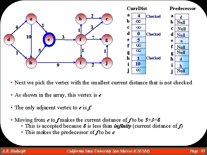
b a 1 4 10 d 3 h 7 f 1 5 1 9 c 3 1 e 2 i g 1 2 j Curr. Dist a 4 Checked b c d 0 Checked e 5 f g h 1 Checked i 10 j Predecessor a d b Null c Null d Null e a f Null g Null h d i h j Null • Next we pick the vertex with the smallest current distance that is not checked • As shown in the array, this vertex is e • The only adjacent vertex to e is f. • Moving from e to f makes the current distance of f to be 5+3=8 • This is accepted because 8 is less than infinity (current distance of f) • This makes the predecessor of f to be e A. R. Hadaegh Dr. Ahmad R. Hadaegh California State University San Marcos (CSUSM) Page 43

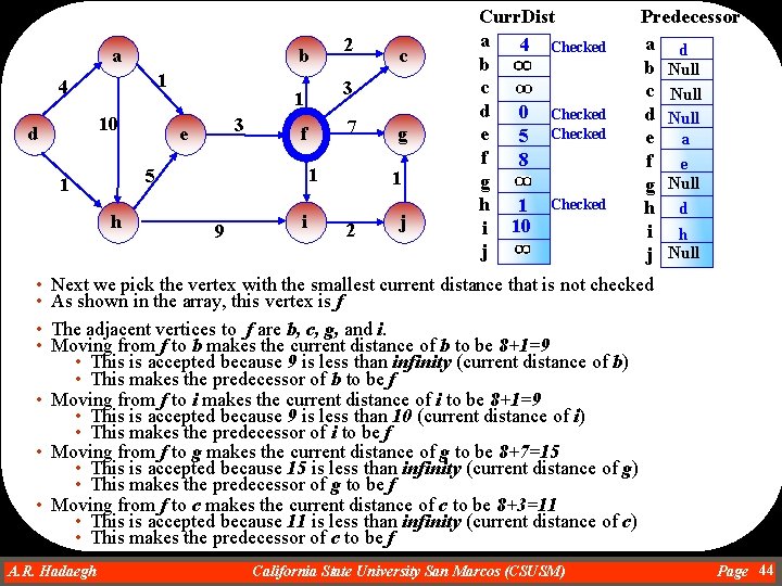
b a 1 4 10 d 3 h 7 f 1 5 1 9 i c 3 1 e 2 g 1 2 j Curr. Dist a 4 Checked b c d 0 Checked e 5 Checked f 8 g h 1 Checked i 10 j Predecessor a d b Null c Null d Null e a f e g Null h d i h j Null • • Next we pick the vertex with the smallest current distance that is not checked As shown in the array, this vertex is f The adjacent vertices to f are b, c, g, and i. Moving from f to b makes the current distance of b to be 8+1=9 • This is accepted because 9 is less than infinity (current distance of b) • This makes the predecessor of b to be f • Moving from f to i makes the current distance of i to be 8+1=9 • This is accepted because 9 is less than 10 (current distance of i) • This makes the predecessor of i to be f • Moving from f to g makes the current distance of g to be 8+7=15 • This is accepted because 15 is less than infinity (current distance of g) • This makes the predecessor of g to be f • Moving from f to c makes the current distance of c to be 8+3=11 • This is accepted because 11 is less than infinity (current distance of c) • This makes the predecessor of c to be f A. R. Hadaegh Dr. Ahmad R. Hadaegh California State University San Marcos (CSUSM) Page 44

a 1 4 10 d 3 e h 7 f 1 9 c 3 1 5 1 2 b i g 1 2 j Curr. Dist a 4 Checked b 9 c 11 d 0 Checked e 5 Checked f 8 Checked g 15 h 1 Checked 9 i j Predecessor a d b f c f d Null e a f e g f h d i f j Null • Next we pick the vertex with the smallest current distance that is not checked • As shown in the array, this vertex is either b or i. We can pick any of them. So we select b. • The only adjacent vertex to b is c. • Moving from b to c makes the current distance of c to be 9+2=11 • This is not accepted because 11 is not less than 11 (current distance of c) A. R. Hadaegh Dr. Ahmad R. Hadaegh California State University San Marcos (CSUSM) Page 45

a b 1 4 10 d 3 h 7 f 1 5 1 9 c 3 1 e 2 i g 1 2 j Curr. Dist a 4 Checked b 9 Checked c 11 d 0 Checked e 5 Checked f 8 Checked g 15 h 1 Checked 9 i j Predecessor a d b f c f d Null e a f e g f h d i f j Null • Next we pick the vertex with the smallest current distance that is not checked • As shown in the array, this vertex is i. • The only adjacent vertex to i is j. • Moving from i to j makes the current distance of j to be 9+2=11 • This is accepted because 11 is less than infinity (current distance of j) • This makes the predecessor of j to be i A. R. Hadaegh Dr. Ahmad R. Hadaegh California State University San Marcos (CSUSM) Page 46

a b 1 4 10 d 3 h 7 f 1 5 1 9 c 3 1 e 2 i g 1 2 j Curr. Dist a 4 Checked b 9 Checked c 11 d 0 Checked e 5 Checked f 8 Checked g 15 h 1 Checked 9 Checked i j 11 Predecessor a d b f c f d Null e a f e g f h d i f j i • Next we pick the vertex with the smallest current distance that is not checked • As shown in the array, this vertex is either c or j. We select c • There is no adjacent vertex to c A. R. Hadaegh Dr. Ahmad R. Hadaegh California State University San Marcos (CSUSM) Page 47

a b 1 4 10 d 3 h 7 f 1 5 1 9 c 3 1 e 2 i g 1 2 j Curr. Dist a 4 Checked b 9 Checked c 11 Checked d 0 Checked e 5 Checked f 8 Checked g 15 h 1 Checked 9 Checked i j 11 Predecessor a d b f c f d Null e a f e g f h d i f j i • Next we pick the vertex with the smallest current distance that is not checked • As shown in the array, this vertex is j. • The only adjacent vertex to j is g. • Moving from j to g makes the current distance of g to be 11+1=12 • This is accepted because 12 is less than 15 (current distance of g) • This makes the predecessor of g to be j A. R. Hadaegh Dr. Ahmad R. Hadaegh California State University San Marcos (CSUSM) Page 48

a b 1 4 10 d 3 h 7 f 1 5 1 9 c 3 1 e 2 i g 1 2 j Curr. Dist a 4 Checked b 9 Checked c 11 Checked d 0 Checked e 5 Checked f 8 Checked g 12 h 1 Checked 9 Checked i j 11 Checked Predecessor a d b f c f d Null e a f e g j h d i f j i • Next we pick the vertex with the smallest current distance that is not checked • As shown in the array, this vertex is g. • There is no adjacent vertex to g A. R. Hadaegh Dr. Ahmad R. Hadaegh California State University San Marcos (CSUSM) Page 49

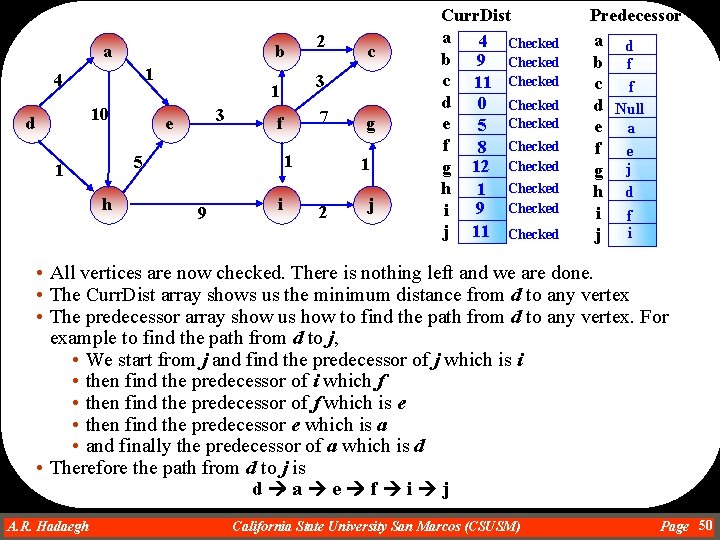
a b 1 4 10 d 3 h 7 f 1 5 1 9 i c 3 1 e 2 g 1 2 j Curr. Dist a 4 Checked b 9 Checked c 11 Checked d 0 Checked e 5 Checked f 8 Checked g 12 Checked h 1 Checked 9 Checked i j 11 Checked Predecessor a d b f c f d Null e a f e g j h d i f j i • All vertices are now checked. There is nothing left and we are done. • The Curr. Dist array shows us the minimum distance from d to any vertex • The predecessor array show us how to find the path from d to any vertex. For example to find the path from d to j, • We start from j and find the predecessor of j which is i • then find the predecessor of i which f • then find the predecessor of f which is e • then find the predecessor e which is a • and finally the predecessor of a which is d • Therefore the path from d to j is d a e f i j A. R. Hadaegh Dr. Ahmad R. Hadaegh California State University San Marcos (CSUSM) Page 50

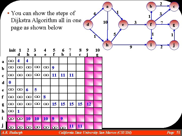
a • You can show the steps of Dijkstra Algorithm all in one page as shown below 1 4 10 d h a 2 3 h a 4 4 e 5 f 6 b 7 i b 9 c 11 11 11 8 c 9 j 10 g 3 e 2 7 f 1 9 i c 3 1 5 1 init 1 d 4 b g 1 2 j d 0 6 e 5 f 8 g h i 15 15 12 1 10 10 10 9 j A. R. Hadaegh Dr. Ahmad R. Hadaegh 9 11 11 California State University San Marcos (CSUSM) Page 51

Complexity of Dijkstra Algorithm • The complexity of Dijkstra algorithm is O(|V 2|) • The first for loop and the while loop are executed |V| times • For each iteration of the while loop • A vertex in to. Be. Checked list with minimal current distance has to be found which requires O(|V|) steps • The for loop iterates deg(v) times which is also O(|V|) • Problem: • Dijkstra algorithm only works for positive weights and it fails when negative weights are used in graphs A. R. Hadaegh Dr. Ahmad R. Hadaegh California State University San Marcos (CSUSM) Page 52

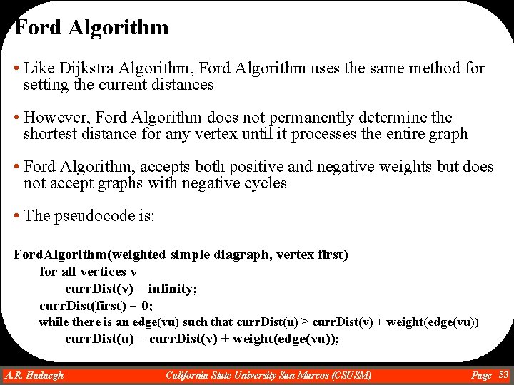
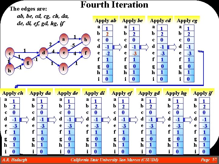
Ford Algorithm • Like Dijkstra Algorithm, Ford Algorithm uses the same method for setting the current distances • However, Ford Algorithm does not permanently determine the shortest distance for any vertex until it processes the entire graph • Ford Algorithm, accepts both positive and negative weights but does not accept graphs with negative cycles • The pseudocode is: Ford. Algorithm(weighted simple diagraph, vertex first) for all vertices v curr. Dist(v) = infinity; curr. Dist(first) = 0; while there is an edge(vu) such that curr. Dist(u) > curr. Dist(v) + weight(edge(vu)) curr. Dist(u) = curr. Dist(v) + weight(edge(vu)); A. R. Hadaegh Dr. Ahmad R. Hadaegh California State University San Marcos (CSUSM) Page 53

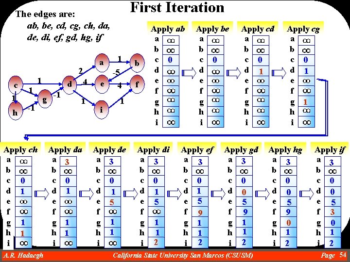
First Iteration The edges are: ab, be, cd, cg, ch, da, de, di, ef, gd, hg, if a 2 c 1 h 1 -1 Apply ch a b c 0 d 1 e f g 1 h 1 i 1 4 d g -1 1 Apply da a 3 b c 0 d 1 e f g 1 h 1 i A. R. Hadaegh Dr. Ahmad R. Hadaegh 1 -5 e i 4 1 Apply de a 3 b c 0 d 1 e 5 f g 1 h 1 i b f Apply ab a b c 0 d e f g h i Apply di a 3 b c 0 d 1 e 5 f g 1 h 1 i 2 Apply be a b c 0 d e f g h i Apply ef a 3 b c 0 d 1 e 5 f 9 g 1 h 1 i 2 Apply cd a b c 0 d 1 e f g h i Apply gd a 3 b c 0 d 0 e 5 f 9 g 1 h 1 i 2 California State University San Marcos (CSUSM) Apply cg a b c 0 d 1 e f g 1 h i Apply hg a 3 b c 0 d 0 e 5 f 9 g 0 h 1 i 2 Apply if a 3 b c 0 d 0 e 5 f 3 g 0 h 1 i 2 Page 54

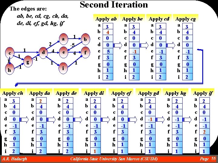
Second Iteration The edges are: ab, be, cd, cg, ch, da, de, di, ef, gd, hg, if a 2 c 1 h 1 -1 Apply ch a 3 b 4 c 0 d 0 e -1 f 3 g 0 h 1 i 2 1 d g -1 Apply da a 2 b 4 c 0 d 0 e -1 f 3 g 0 h 1 i 2 A. R. Hadaegh Dr. Ahmad R. Hadaegh 4 1 1 -5 e i 4 1 Apply de a 2 b 4 c 0 d 0 e -1 f 3 g 0 h 1 i 2 b f Apply ab Apply be a 3 b 4 c 0 d 0 e 5 e -1 f 3 g 0 h 1 i 2 Apply di a 2 b 4 c 0 d 0 e -1 f 3 g 0 h 1 i 1 Apply ef a 2 b 4 c 0 d 0 e -1 f 3 g 0 h 1 i 1 Apply cd a 3 b 4 c 0 d 0 e -1 f 3 g 0 h 1 i 2 Apply gd a 2 b 4 c 0 d -1 e -1 f 3 g 0 h 1 i 1 California State University San Marcos (CSUSM) Apply cg a 3 b 4 c 0 d 0 e -1 f 3 g 0 h 1 i 2 Apply hg a 2 b 4 c 0 d -1 e -1 f 3 g 0 h 1 i 1 Apply if a 2 b 4 c 0 d -1 e -1 f 2 g 0 h 1 i 1 Page 55

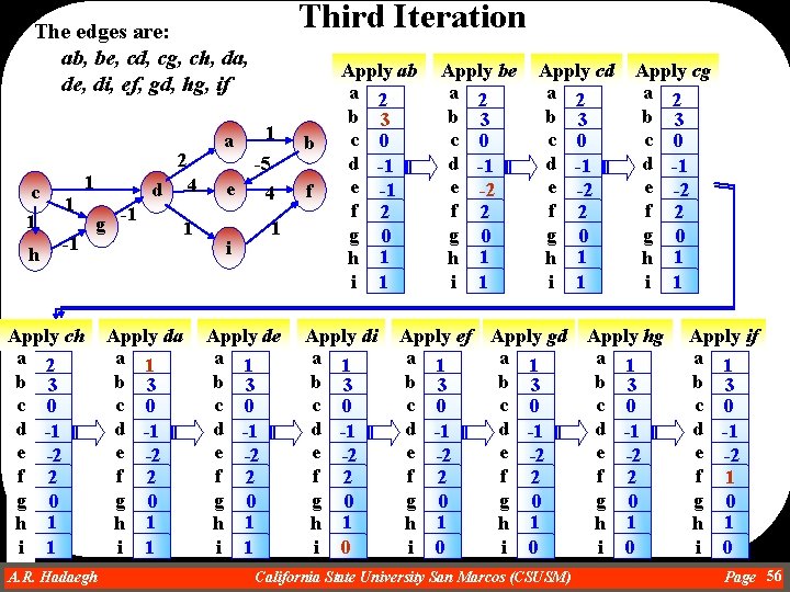
Third Iteration The edges are: ab, be, cd, cg, ch, da, de, di, ef, gd, hg, if a 2 c 1 h 1 -1 Apply ch a 2 b 3 c 0 d -1 e -2 f 2 g 0 h 1 i 1 1 d g -1 Apply da a 1 b 3 c 0 d -1 e -2 f 2 g 0 h 1 i 1 A. R. Hadaegh Dr. Ahmad R. Hadaegh 4 1 1 -5 e i 4 1 Apply de a 1 b 3 c 0 d -1 e -2 f 2 g 0 h 1 i 1 b f Apply ab a 2 b 3 c 0 d -1 e -1 f 2 g 0 h 1 i 1 Apply di a 1 b 3 c 0 d -1 e -2 f 2 g 0 h 1 i 0 Apply be a 2 b 3 c 0 d -1 e -2 f 2 g 0 h 1 i 1 Apply cd a 2 b 3 c 0 d -1 e -2 f 2 g 0 h 1 i 1 Apply cg a 2 b 3 c 0 d -1 e -2 f 2 g 0 h 1 i 1 Apply ef Apply gd Apply hg a 1 a 1 b 3 b 3 c 0 c 0 d -1 e -2 f 2 f 2 g 0 g 0 h 1 h 1 i 0 i 0 California State University San Marcos (CSUSM) Apply if a 1 b 3 c 0 d -1 e -2 f 1 g 0 h 1 i 0 Page 56

Fourth Iteration The edges are: ab, be, cd, cg, ch, da, de, di, ef, gd, hg, if a 2 c 1 h 1 -1 Apply ch a 1 b 2 c 0 d -1 e -3 f 1 g 0 h 1 i 0 1 d g -1 Apply da a 1 b 2 c 0 d -1 e -3 f 1 g 0 h 1 i 0 A. R. Hadaegh Dr. Ahmad R. Hadaegh 4 1 1 -5 e i 4 1 Apply de a 1 b 2 c 0 d -1 e -3 f 1 g 0 h 1 i 0 b f Apply ab a 1 b 2 c 0 d -1 e -2 f 1 g 0 h 1 i 0 Apply di a 1 b 2 c 0 d -1 e -3 f 1 g 0 h 1 i 0 Apply be a 1 b 2 c 0 d -1 e -3 f 1 g 0 h 1 i 0 Apply ef a 1 b 2 c 0 d -1 e -3 f 1 g 0 h 1 i 0 Apply cd a 1 b 2 c 0 d -1 e -3 f 1 g 0 h 1 i 0 Apply gd a 1 b 2 c 0 d -1 e -3 f 1 g 0 h 1 i 0 California State University San Marcos (CSUSM) Apply cg a 1 b 2 c 0 d -1 e -3 f 1 g 0 h 1 i 0 Apply hg a 1 b 2 c 0 d -1 e -3 f 1 g 0 h 1 i 0 Apply if a 1 b 2 c 0 d -1 e -3 f 1 g 0 h 1 i 0 Page 57

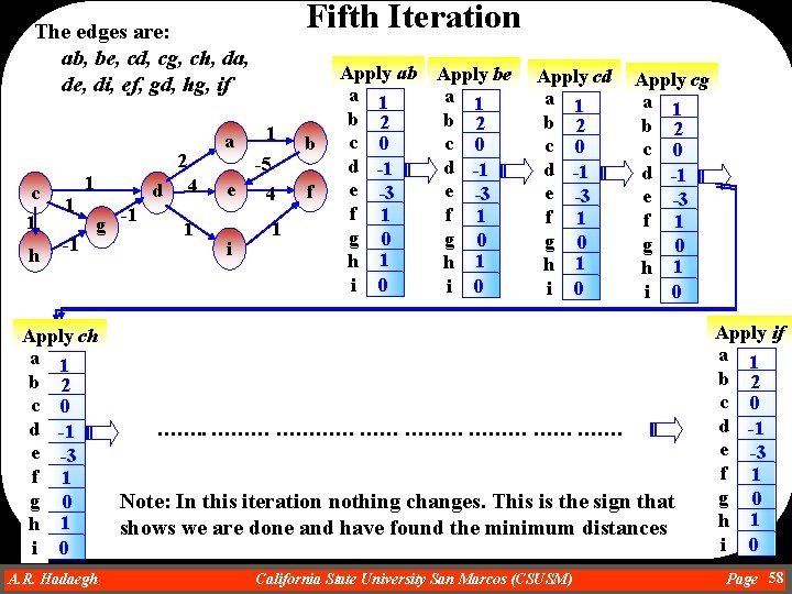
Fifth Iteration The edges are: ab, be, cd, cg, ch, da, de, di, ef, gd, hg, if a 2 c 1 h 1 -1 1 d g -1 Apply ch a 1 b 2 c 0 d -1 e -3 f 1 g 0 h 1 i 0 4 1 1 -5 e i 4 1 b f Apply ab Apply be a 1 b 2 c 0 d -1 e -3 f 1 g 0 h 1 i 0 Apply cd a 1 b 2 c 0 d -1 e -3 f 1 g 0 h 1 i 0 Apply cg a 1 b 2 c 0 d -1 e -3 f 1 g 0 h 1 i 0 ……. . ………… …… ……. Note: In this iteration nothing changes. This is the sign that shows we are done and have found the minimum distances A. R. Hadaegh Dr. Ahmad R. Hadaegh California State University San Marcos (CSUSM) Apply if a 1 b 2 c 0 d -1 e -3 f 1 g 0 h 1 i 0 Page 58

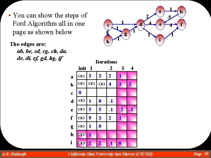
• In the example of the Ford algorithm, we ordered the edges alphabetically. However, the order of the edges should have no effect on the final result • In this example, we showed that we do as many as iterations as required in order to find the minimum distance from the source vertex (called first in the algorithm) to any other vertex. • Note that the current distance of some vertices changed more than once even within the same iteration A. R. Hadaegh Dr. Ahmad R. Hadaegh California State University San Marcos (CSUSM) Page 59

Complexity of Ford Algorithm • The computational complexity of this algorithm is O(|V|*|E|) because • there would be at most |V| - 1 passes through the sequence of |E| edges since |V| -1 is the largest number of edges in any path • in the first pass, at least one-edge paths are determined • in the second pass, all two-edges paths are determined • and so on A. R. Hadaegh Dr. Ahmad R. Hadaegh California State University San Marcos (CSUSM) Page 60

• You can show the steps of Ford Algorithm all in one page as shown below The edges are: ab, be, cd, cg, ch, da, de, di, ef, gd, hg, if 2 c 1 1 1 -1 h d g -1 4 1 1 -5 e i 4 b f 1 Iterations init 1 2 3 4 3 3 2 1 a 4 3 2 b c A. R. Hadaegh Dr. Ahmad R. Hadaegh a 0 d 1 0 -1 e 5 5 -1 -2 f 9 3 2 1 g 1 0 h 1 i 2 1 0 2 -3 California State University San Marcos (CSUSM) Page 61

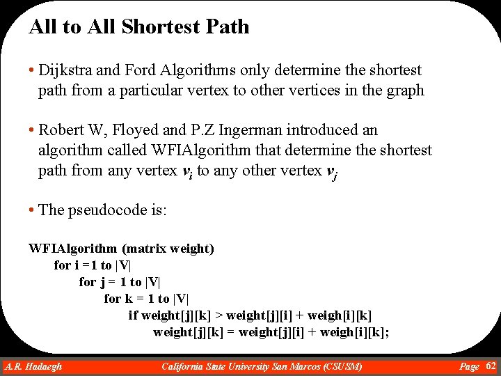
All to All Shortest Path • Dijkstra and Ford Algorithms only determine the shortest path from a particular vertex to other vertices in the graph • Robert W, Floyed and P. Z Ingerman introduced an algorithm called WFIAlgorithm that determine the shortest path from any vertex vi to any other vertex vj • The pseudocode is: WFIAlgorithm (matrix weight) for i =1 to |V| for j = 1 to |V| for k = 1 to |V| if weight[j][k] > weight[j][i] + weigh[i][k] weight[j][k] = weight[j][i] + weigh[i][k]; A. R. Hadaegh Dr. Ahmad R. Hadaegh California State University San Marcos (CSUSM) Page 62

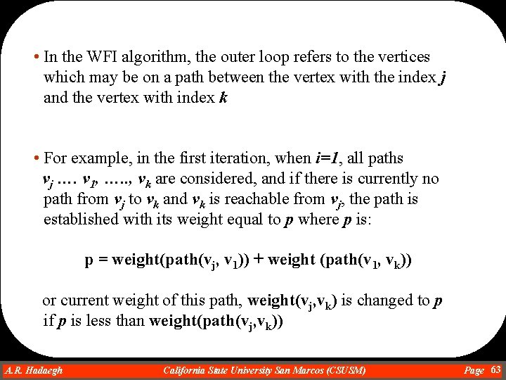
• In the WFI algorithm, the outer loop refers to the vertices which may be on a path between the vertex with the index j and the vertex with index k • For example, in the first iteration, when i=1, all paths vj …. v 1, …. . , vk are considered, and if there is currently no path from vj to vk and vk is reachable from vj, the path is established with its weight equal to p where p is: p = weight(path(vj, v 1)) + weight (path(v 1, vk)) or current weight of this path, weight(vj, vk) is changed to p if p is less than weight(path(vj, vk)) A. R. Hadaegh Dr. Ahmad R. Hadaegh California State University San Marcos (CSUSM) Page 63

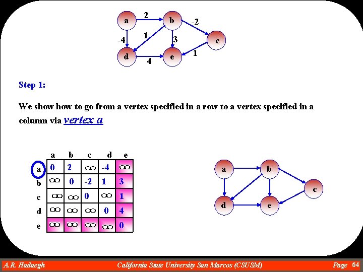
a -4 d 2 1 4 b -2 3 e c 1 Step 1: We show to go from a vertex specified in a row to a vertex specified in a column via vertex a b a 0 b 2 c 0 -2 c d e A. R. Hadaegh Dr. Ahmad R. Hadaegh a d -4 1 0 e a 3 1 0 b 4 c d e 0 California State University San Marcos (CSUSM) Page 64

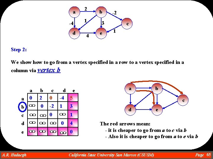
a -4 d 2 1 4 b -2 3 e c 1 Step 2: We show to go from a vertex specified in a row to a vertex specified in a column via vertex a b a 0 b b 2 c 0 d e -4 5 0 -2 1 c d e A. R. Hadaegh Dr. Ahmad R. Hadaegh 0 3 1 0 4 0 a b c d e The red arrows mean: - it is cheaper to go from a to c via b - Also it is cheaper to go from a to e via b California State University San Marcos (CSUSM) Page 65

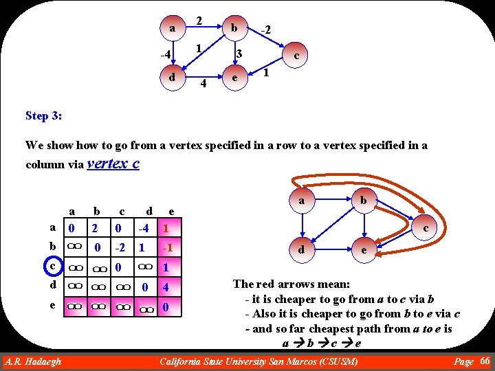
a -4 d 2 1 4 b -2 3 e c 1 Step 3: We show to go from a vertex specified in a row to a vertex specified in a column via vertex a b a 0 c b 2 c 0 d e -4 1 0 -2 1 c d e A. R. Hadaegh Dr. Ahmad R. Hadaegh 0 -1 a b c d e 1 0 4 0 The red arrows mean: - it is cheaper to go from a to c via b - Also it is cheaper to go from b to e via c - and so far cheapest path from a to e is a b c e California State University San Marcos (CSUSM) Page 66

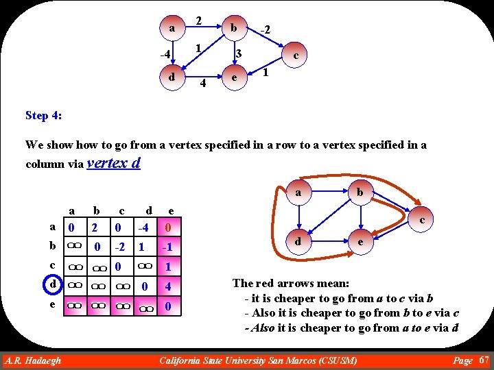
a -4 d 2 1 4 b -2 3 e c 1 Step 4: We show to go from a vertex specified in a row to a vertex specified in a column via vertex d a a b a 0 b 2 c 0 d -4 e 0 0 -2 1 -1 c d e A. R. Hadaegh Dr. Ahmad R. Hadaegh 0 b c d e 1 0 4 0 The red arrows mean: - it is cheaper to go from a to c via b - Also it is cheaper to go from b to e via c - Also it is cheaper to go from a to e via d California State University San Marcos (CSUSM) Page 67

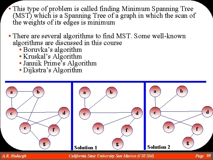
Spanning Trees • Consider a graph that represents airline connection • If economic situation forces this airline to shut down as many connection as possible, which of them should be retained to make sure that it is still possible to reach any city from other cities • The point is to find a solution that allows us to remove as many edges as possible such that any node can be reached from any other node • You may be able to find several solutions to this problem; however, if there is cost involved in going from node A to node B , then we prefer to minimize the number of connections with the lowest cost possible A. R. Hadaegh Dr. Ahmad R. Hadaegh California State University San Marcos (CSUSM) Page 68

• This type of problem is called finding Minimum Spanning Tree (MST) which is a Spanning Tree of a graph in which the scan of the weights of its edges is minimum • There are several algorithms to find MST. Some well-known algorithms are discussed in this course • Boruvka’s algorithm • Kruskal’s Algorithm • Jannik Prime’s Algorithm • Dijkstra’s Algorithm b a a d c e f g A. R. Hadaegh Dr. Ahmad R. Hadaegh a b d c e Solution 1 d c e f g b Solution 2 California State University San Marcos (CSUSM) f g Page 69

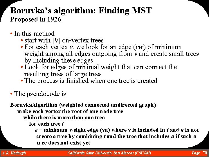
Boruvka’s algorithm: Finding MST Proposed in 1926 • In this method • start with |V| on-vertex trees • For each vertex v, we look for an edge (vw) of minimum weight among all edges outgoing from v and create small trees by including these edges • Look for edges of minimal weight that can connect the resulting trees of large trees • The process is finished when one tree is created • The pseudocode is: Boruvka. Algorithm (weighted connected undirected graph) make each vertex the root of one-node tree while there is more than one tree for each tree t e = minimum weight edge (vu) where v is included in t and u is not create a tree by combining t and the tree that includes u if such a tree does not exist yet A. R. Hadaegh Dr. Ahmad R. Hadaegh California State University San Marcos (CSUSM) Page 70

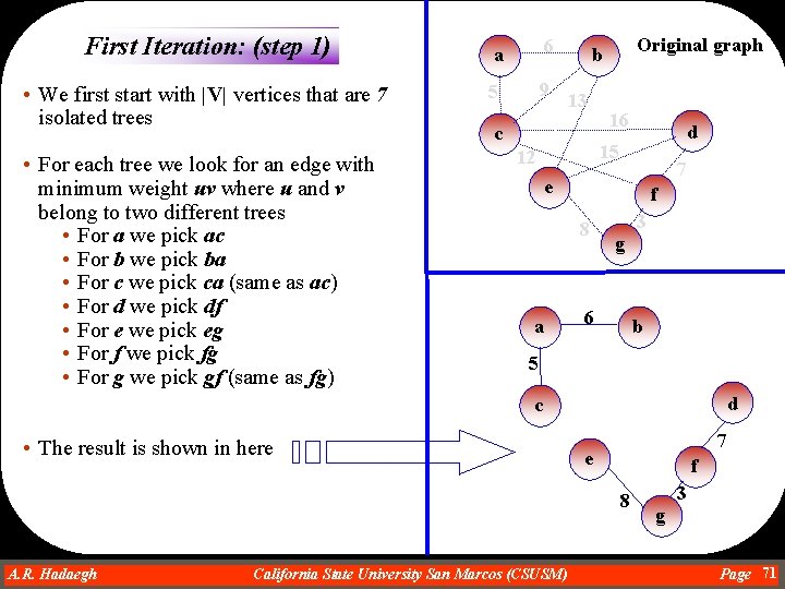
First Iteration: (step 1) • We first start with |V| vertices that are 7 isolated trees • For each tree we look for an edge with minimum weight uv where u and v belong to two different trees • For a we pick ac • For b we pick ba • For c we pick ca (same as ac) • For d we pick df • For e we pick eg • For f we pick fg • For g we pick gf (same as fg) a 6 5 9 Original graph b 13 c 16 d 15 12 7 e f 8 a 3 g 6 b 5 d c • The result is shown in here 7 e f 8 A. R. Hadaegh Dr. Ahmad R. Hadaegh California State University San Marcos (CSUSM) 3 g Page 71

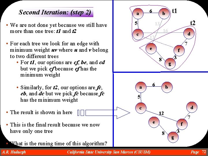
Second Iteration: (step 2) a • We are not done yet because we still have more than one tree: t 1 and t 2 5 6 • The result is shown in here t 2 13 16 c d 12 • For each tree we look for an edge with minimum weight uv where u and v belong to two different trees • For t 1, our options are cf, be, and cd but we pick cf because cf has the minimum weight • Similarly, for t 2, our options are fc, eb, and dc but we pick fc because fc has the minimum weight t 1 b 7 e f 3 8 a g 6 b 5 d c • This is the final result because we now have only one tree 12 7 e f 8 3 g • What is the runing time of this algorithm? A. R. Hadaegh Dr. Ahmad R. Hadaegh California State University San Marcos (CSUSM) Page 72

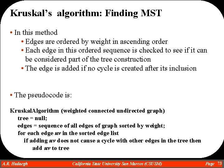
Kruskal’s algorithm: Finding MST • In this method • Edges are ordered by weight in ascending order • Each edge in this ordered sequence is checked to see if it can be considered part of the tree construction • The edge is added if no cycle is created after its inclusion • The pseudocode is: Kruskal. Algorithm (weighted connected undirected graph) tree = null; edges = sequence of all edges of graph sorted by weight; for each edge uv in the sorted edge list if adding uv does not cause a cycle with other edges in the tree then add uv to tree A. R. Hadaegh Dr. Ahmad R. Hadaegh California State University San Marcos (CSUSM) Page 73

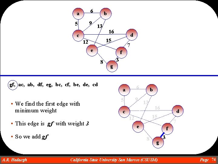
a 6 5 9 b 13 c 16 d 15 12 7 e f 8 gf, ac, ab, df, eg, bc, cf, be, de, cd • We find the first edge with minimum weight • This edge is gf with weight 3 • So we add gf A. R. Hadaegh Dr. Ahmad R. Hadaegh 3 g a 6 5 9 b 13 c 16 d 15 12 7 e f 8 g California State University San Marcos (CSUSM) 3 Page 74

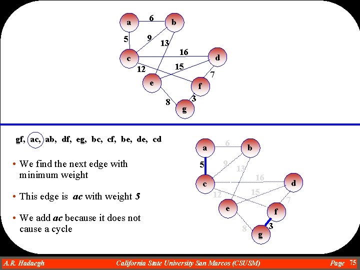
a 6 5 9 b 13 c 16 d 15 12 7 e f 8 gf, ac, ab, df, eg, bc, cf, be, de, cd • We find the next edge with minimum weight • This edge is ac with weight 5 • We add ac because it does not cause a cycle A. R. Hadaegh Dr. Ahmad R. Hadaegh 3 g a 6 5 9 b 13 c 16 d 15 12 7 e f 8 g California State University San Marcos (CSUSM) 3 Page 75

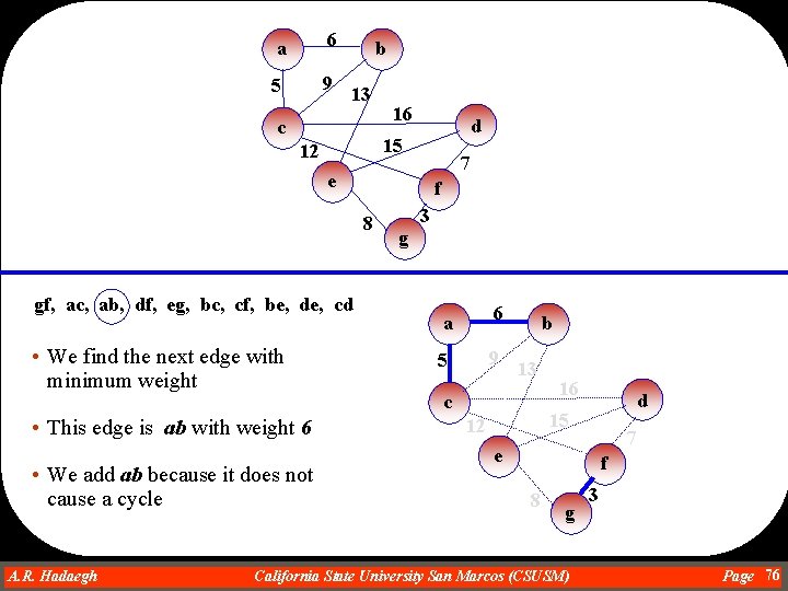
a 6 5 9 b 13 c 16 d 15 12 7 e f 8 gf, ac, ab, df, eg, bc, cf, be, de, cd • We find the next edge with minimum weight • This edge is ab with weight 6 • We add ab because it does not cause a cycle A. R. Hadaegh Dr. Ahmad R. Hadaegh 3 g a 6 5 9 b 13 c 16 d 15 12 7 e f 8 g California State University San Marcos (CSUSM) 3 Page 76

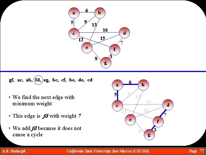
a 6 5 9 b 13 c 16 d 15 12 7 e f 8 gf, ac, ab, fd, eg, bc, cf, be, de, cd • We find the next edge with minimum weight • This edge is fd with weight 7 • We add fd because it does not cause a cycle A. R. Hadaegh Dr. Ahmad R. Hadaegh 3 g a 6 5 9 b 13 c 16 d 15 12 7 e f 8 g California State University San Marcos (CSUSM) 3 Page 77

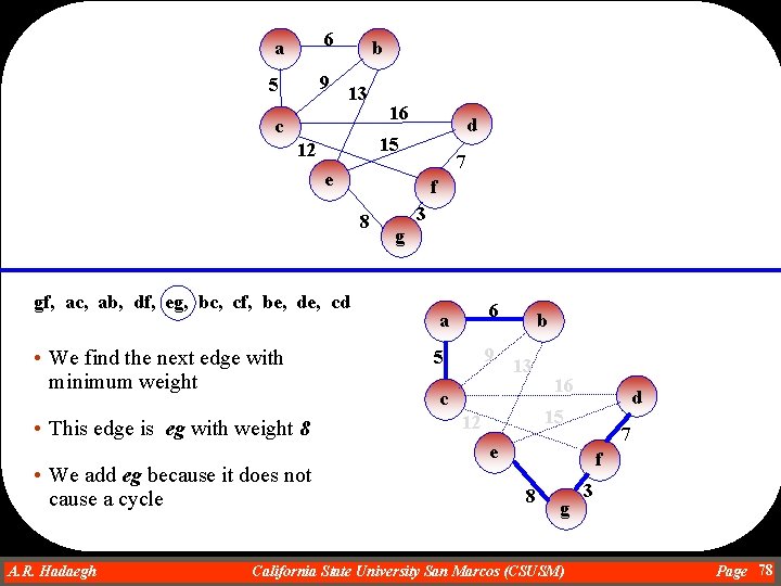
a 6 5 9 b 13 c 16 d 15 12 7 e f 8 gf, ac, ab, df, eg, bc, cf, be, de, cd • We find the next edge with minimum weight • This edge is eg with weight 8 • We add eg because it does not cause a cycle A. R. Hadaegh Dr. Ahmad R. Hadaegh 3 g a 6 5 9 b 13 c 16 d 15 12 7 e f 8 g California State University San Marcos (CSUSM) 3 Page 78

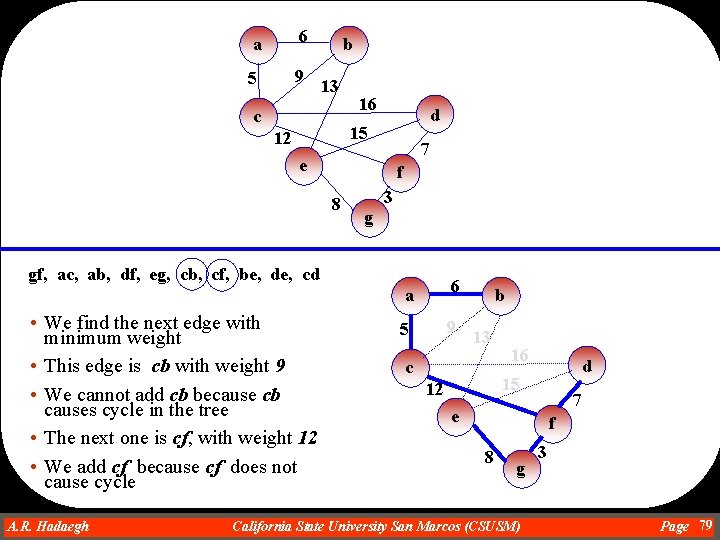
a 6 5 9 b 13 c 16 d 15 12 7 e f 8 3 g gf, ac, ab, df, eg, cb, cf, be, de, cd • We find the next edge with minimum weight • This edge is cb with weight 9 • We cannot add cb because cb causes cycle in the tree • The next one is cf, with weight 12 • We add cf because cf does not cause cycle A. R. Hadaegh Dr. Ahmad R. Hadaegh a 6 5 9 b 13 c 16 d 15 12 7 e f 8 g California State University San Marcos (CSUSM) 3 Page 79

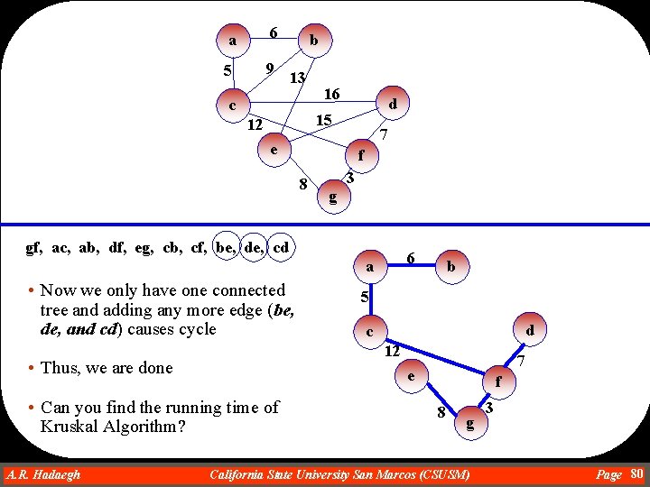
a 6 5 9 b 13 c 16 d 15 12 7 e f 8 3 g gf, ac, ab, df, eg, cb, cf, be, de, cd 6 a • Now we only have one connected tree and adding any more edge (be, de, and cd) causes cycle 5 d c 12 • Thus, we are done 7 e • Can you find the running time of Kruskal Algorithm? A. R. Hadaegh Dr. Ahmad R. Hadaegh b f 8 g California State University San Marcos (CSUSM) 3 Page 80

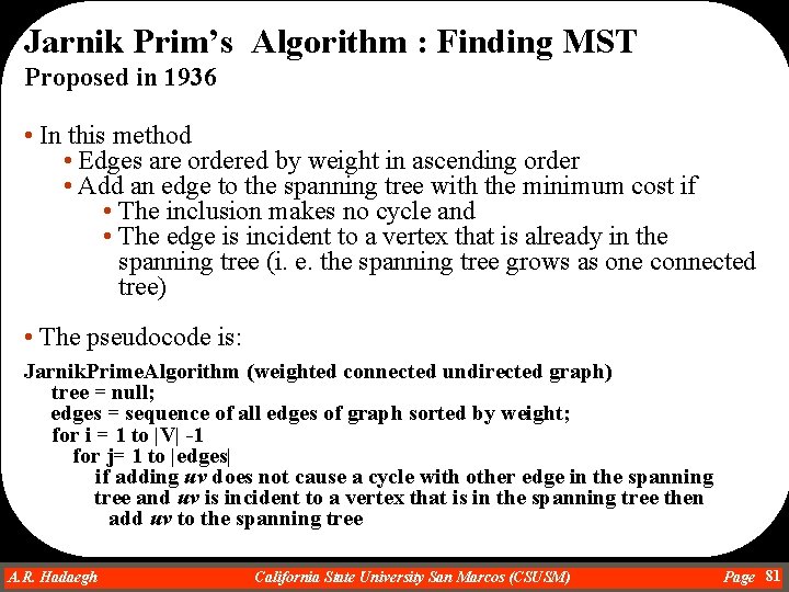
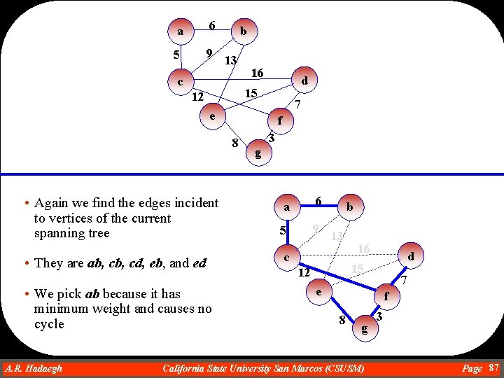
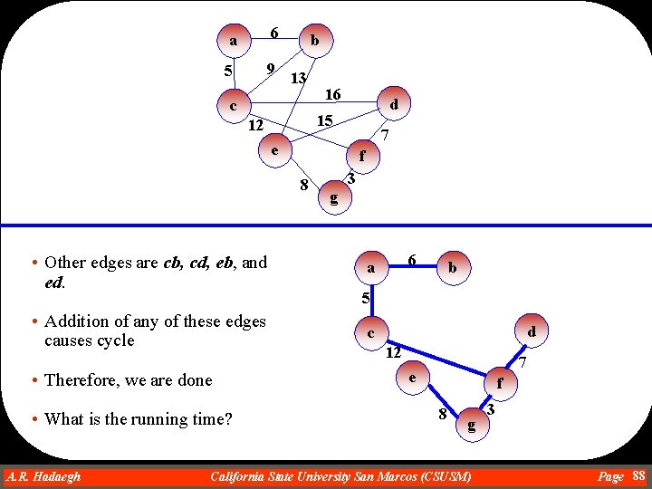
Jarnik Prim’s Algorithm : Finding MST Proposed in 1936 • In this method • Edges are ordered by weight in ascending order • Add an edge to the spanning tree with the minimum cost if • The inclusion makes no cycle and • The edge is incident to a vertex that is already in the spanning tree (i. e. the spanning tree grows as one connected tree) • The pseudocode is: Jarnik. Prime. Algorithm (weighted connected undirected graph) tree = null; edges = sequence of all edges of graph sorted by weight; for i = 1 to |V| -1 for j= 1 to |edges| if adding uv does not cause a cycle with other edge in the spanning tree and uv is incident to a vertex that is in the spanning tree then add uv to the spanning tree A. R. Hadaegh Dr. Ahmad R. Hadaegh California State University San Marcos (CSUSM) Page 81

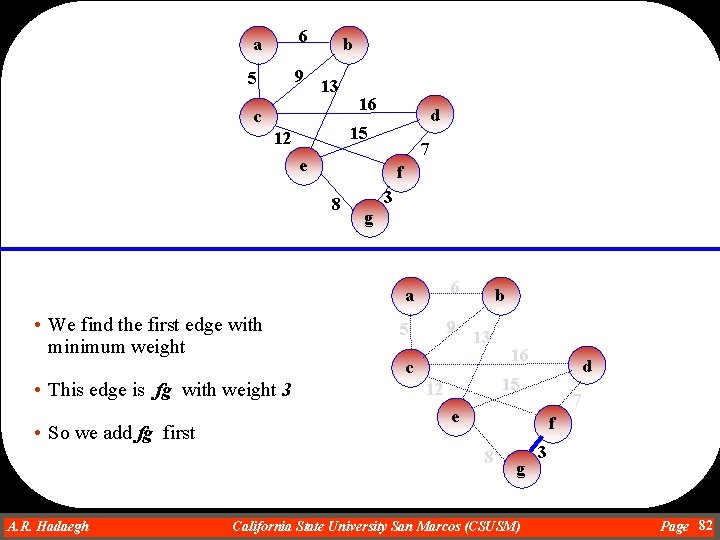
a 6 5 9 b 13 c 16 d 15 12 7 e f 8 • We find the first edge with minimum weight 3 g a 6 5 9 b 13 c • This edge is fg with weight 3 • So we add fg first d 15 12 7 e f 8 A. R. Hadaegh Dr. Ahmad R. Hadaegh 16 g California State University San Marcos (CSUSM) 3 Page 82

a 6 5 9 b 13 c 16 d 15 12 7 e f 8 • Next we find the edges incident to gf. • They are, ge, fc and fd g a 6 5 9 b 13 c • We pick fd because it has minimum weight and causes no cycle A. R. Hadaegh Dr. Ahmad R. Hadaegh 3 16 d 15 12 7 e f 8 g California State University San Marcos (CSUSM) 3 Page 83

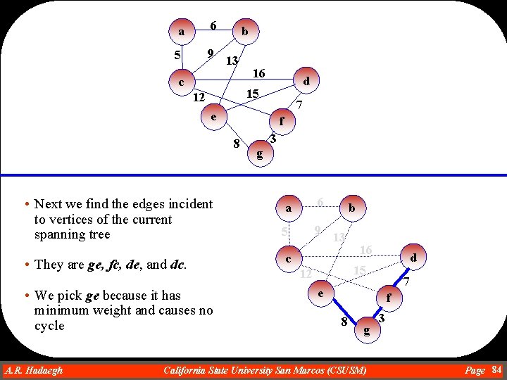
a 6 5 9 b 13 c 16 d 15 12 7 e f 8 • Next we find the edges incident to vertices of the current spanning tree • They are ge, fc, de, and dc. • We pick ge because it has minimum weight and causes no cycle A. R. Hadaegh Dr. Ahmad R. Hadaegh 3 g a 6 5 9 b 13 c 16 d 15 12 7 e f 8 g California State University San Marcos (CSUSM) 3 Page 84

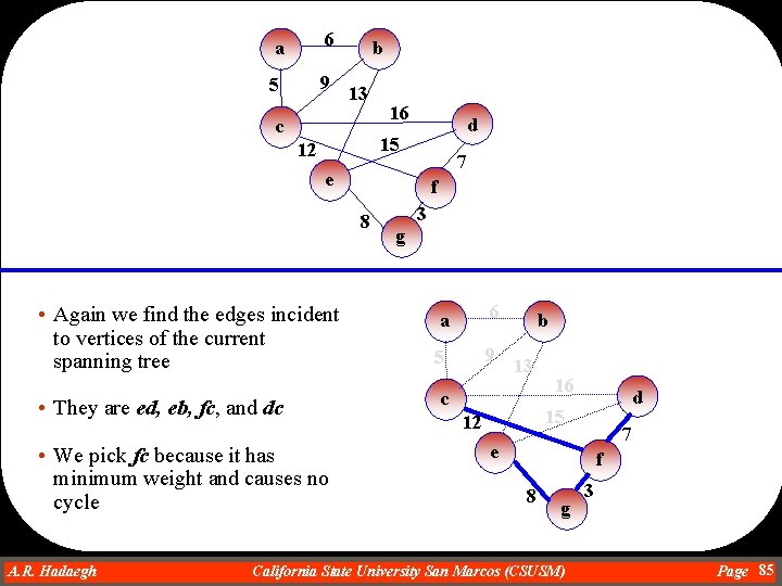
a 6 5 9 b 13 c 16 d 15 12 7 e f 8 • Again we find the edges incident to vertices of the current spanning tree • They are ed, eb, fc, and dc • We pick fc because it has minimum weight and causes no cycle A. R. Hadaegh Dr. Ahmad R. Hadaegh 3 g a 6 5 9 b 13 c 16 d 15 12 7 e f 8 g California State University San Marcos (CSUSM) 3 Page 85

a 6 5 9 b 13 c 16 d 15 12 7 e f 8 • Again we find the edges incident to vertices of the current spanning tree • They are ca, cb, cd, eb, and ed • We pick ca because it has minimum weight and causes no cycle A. R. Hadaegh Dr. Ahmad R. Hadaegh 3 g a 6 5 9 b 13 c 16 d 15 12 7 e f 8 g California State University San Marcos (CSUSM) 3 Page 86

a 6 5 9 b 13 c 16 d 15 12 7 e f 8 • Again we find the edges incident to vertices of the current spanning tree • They are ab, cd, eb, and ed • We pick ab because it has minimum weight and causes no cycle A. R. Hadaegh Dr. Ahmad R. Hadaegh 3 g a 6 5 9 b 13 c 16 d 15 12 7 e f 8 g California State University San Marcos (CSUSM) 3 Page 87

a 6 5 9 b 13 c 16 d 15 12 7 e f 8 • Other edges are cb, cd, eb, and ed. • Addition of any of these edges causes cycle • Therefore, we are done • What is the running time? A. R. Hadaegh Dr. Ahmad R. Hadaegh 3 g 6 a b 5 d c 12 7 e f 8 g California State University San Marcos (CSUSM) 3 Page 88

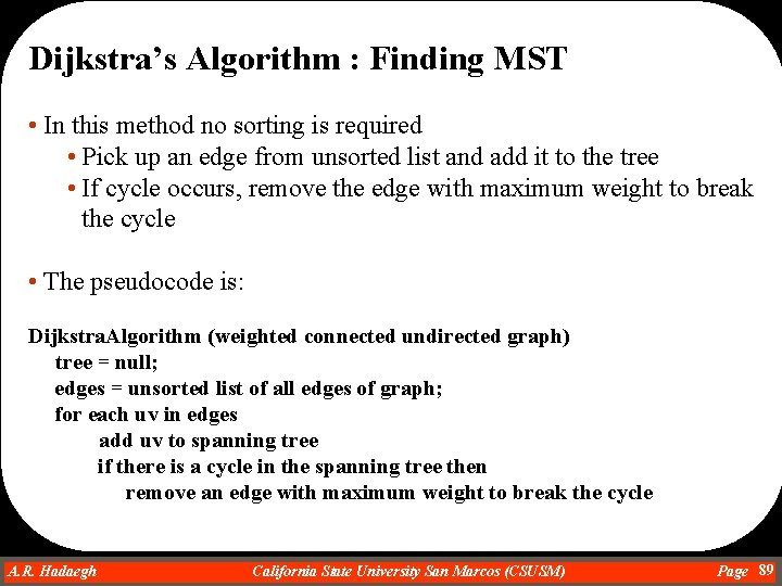
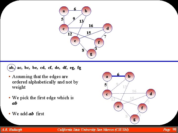
Dijkstra’s Algorithm : Finding MST • In this method no sorting is required • Pick up an edge from unsorted list and add it to the tree • If cycle occurs, remove the edge with maximum weight to break the cycle • The pseudocode is: Dijkstra. Algorithm (weighted connected undirected graph) tree = null; edges = unsorted list of all edges of graph; for each uv in edges add uv to spanning tree if there is a cycle in the spanning tree then remove an edge with maximum weight to break the cycle A. R. Hadaegh Dr. Ahmad R. Hadaegh California State University San Marcos (CSUSM) Page 89

a 6 5 9 b 13 c 16 d 15 12 7 e f 8 3 g ab, ac, be, cd, cf, de, df, eg, fg • Assuming that the edges are ordered alphabetically and not by weight • We pick the first edge which is ab • We add ab first A. R. Hadaegh Dr. Ahmad R. Hadaegh a 6 5 9 b 13 c 16 d 15 12 7 e f 8 California State University San Marcos (CSUSM) g 3 Page 90

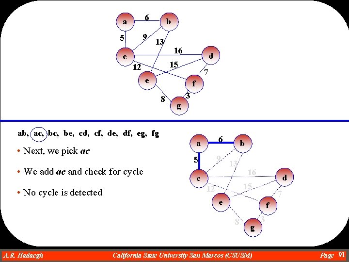
a 6 5 9 b 13 c 16 d 15 12 7 e f 8 3 g ab, ac, be, cd, cf, de, df, eg, fg • Next, we pick ac • We add ac and check for cycle • No cycle is detected a 6 5 9 b 13 c d 15 12 7 e f 8 A. R. Hadaegh Dr. Ahmad R. Hadaegh 16 g California State University San Marcos (CSUSM) 3 Page 91

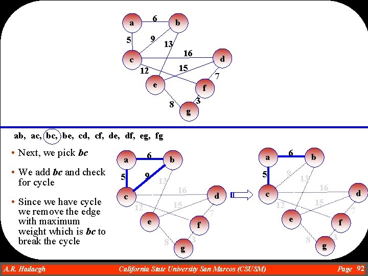
a 6 5 9 b 13 16 c d 15 12 7 e f 3 8 g ab, ac, be, cd, cf, de, df, eg, fg • Next, we pick bc • We add bc and check for cycle • Since we have cycle we remove the edge with maximum weight which is bc to break the cycle A. R. Hadaegh Dr. Ahmad R. Hadaegh a 6 5 9 b 13 c 16 d 15 12 a 6 5 9 f 8 g 13 c 7 e b 3 California State University San Marcos (CSUSM) 16 d 15 12 7 e f 8 g 3 Page 92

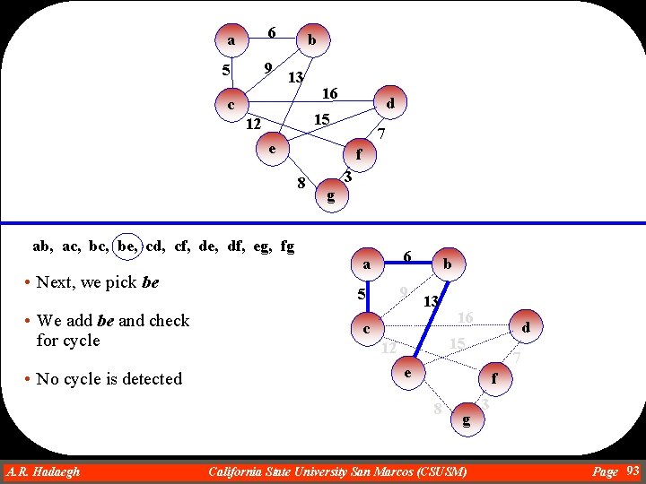
a 6 5 9 b 13 c 16 d 15 12 7 e f 8 3 g ab, ac, be, cd, cf, de, df, eg, fg • Next, we pick be • We add be and check for cycle • No cycle is detected a 6 5 9 b 13 c d 15 12 7 e f 8 A. R. Hadaegh Dr. Ahmad R. Hadaegh 16 g California State University San Marcos (CSUSM) 3 Page 93

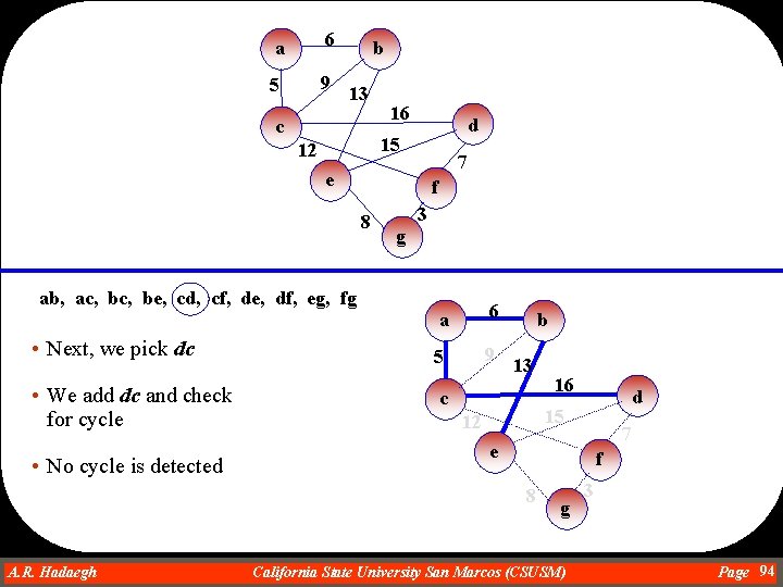
a 6 5 9 b 13 c 16 d 15 12 7 e f 8 3 g ab, ac, be, cd, cf, de, df, eg, fg • Next, we pick dc • We add dc and check for cycle • No cycle is detected a 6 5 9 b 13 c d 15 12 7 e f 8 A. R. Hadaegh Dr. Ahmad R. Hadaegh 16 g California State University San Marcos (CSUSM) 3 Page 94

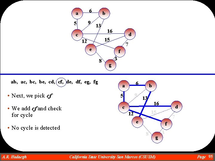
a 6 5 9 b 13 c 16 d 15 12 7 e f 8 ab, ac, be, cd, cf, de, df, eg, fg • Next, we pick cf • We add cf and check for cycle • No cycle is detected A. R. Hadaegh Dr. Ahmad R. Hadaegh 3 g a 6 5 9 b 13 c 16 d 15 12 7 e f 8 g California State University San Marcos (CSUSM) 3 Page 95

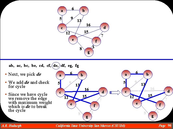
a 6 5 9 b 13 16 c d 15 12 7 e f 3 8 g ab, ac, be, cd, cf, de, df, eg, fg • Next, we pick de a 6 • We add de and check for cycle 5 9 • Since we have cycle we remove the edge with maximum weight which is dc to break the cycle c A. R. Hadaegh Dr. Ahmad R. Hadaegh b 13 16 d 15 12 a 6 5 9 f 8 g 13 c 7 e b 3 California State University San Marcos (CSUSM) 16 d 15 12 7 e f 8 g 3 Page 96

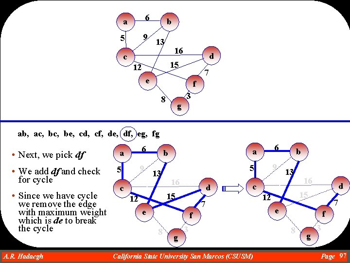
a 6 5 9 b 13 16 c d 15 12 7 e f 3 8 g ab, ac, be, cd, cf, de, df, eg, fg • Next, we pick df a 6 • We add df and check for cycle 5 9 • Since we have cycle we remove the edge with maximum weight which is de to break the cycle A. R. Hadaegh Dr. Ahmad R. Hadaegh b 13 c 16 d 15 12 a 6 5 9 f 8 g 13 c 7 e b 3 California State University San Marcos (CSUSM) 16 d 15 12 7 e f 8 g 3 Page 97

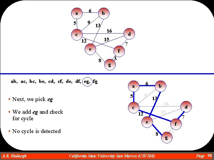
a 6 5 9 b 13 c 16 d 15 12 7 e f 8 ab, ac, be, cd, cf, de, df, eg, fg • Next, we pick eg • We add eg and check for cycle 3 g a 6 5 9 b 13 c d 15 12 7 e • No cycle is detected A. R. Hadaegh Dr. Ahmad R. Hadaegh 16 f 8 California State University San Marcos (CSUSM) g 3 Page 98

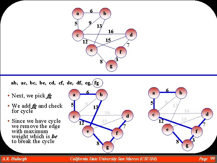
a 6 5 9 b 13 c 16 d 15 12 7 e f 3 8 g ab, ac, be, cd, cf, de, df, eg, fg • Next, we pick fg a 6 • We add fg and check for cycle 5 9 • Since we have cycle we remove the edge with maximum weight which is be to break the cycle A. R. Hadaegh Dr. Ahmad R. Hadaegh b 13 c 16 d 15 12 a 6 5 9 f 8 g 13 c 7 e b 3 California State University San Marcos (CSUSM) 16 d 15 12 7 e f 8 g 3 Page 99

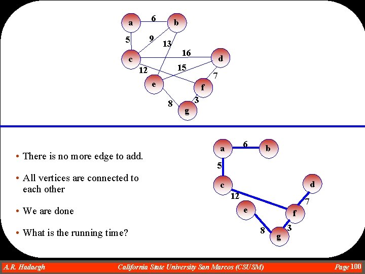
a 6 5 9 b 13 c 16 d 15 12 7 e f 8 • There is no more edge to add. • All vertices are connected to each other g 6 a b 5 d c 12 7 e • We are done • What is the running time? A. R. Hadaegh Dr. Ahmad R. Hadaegh 3 f 8 California State University San Marcos (CSUSM) g 3 Page 100