Graphs Graphs Made up of vertices and arcs

Graphs

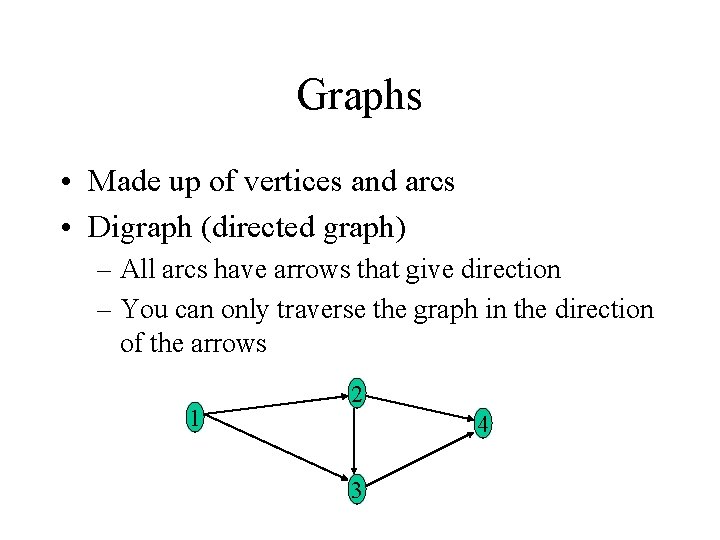
Graphs • Made up of vertices and arcs • Digraph (directed graph) – All arcs have arrows that give direction – You can only traverse the graph in the direction of the arrows 1 2 4 3

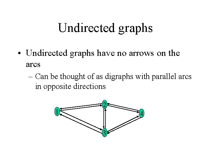
Undirected graphs • Undirected graphs have no arrows on the arcs – Can be thought of as digraphs with parallel arcs in opposite directions 1 2 4 3

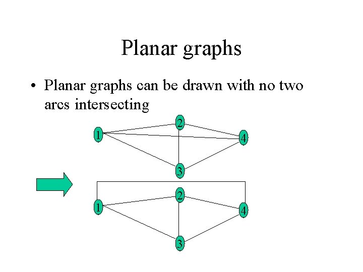
Planar graphs • Planar graphs can be drawn with no two arcs intersecting 1 2 4 3

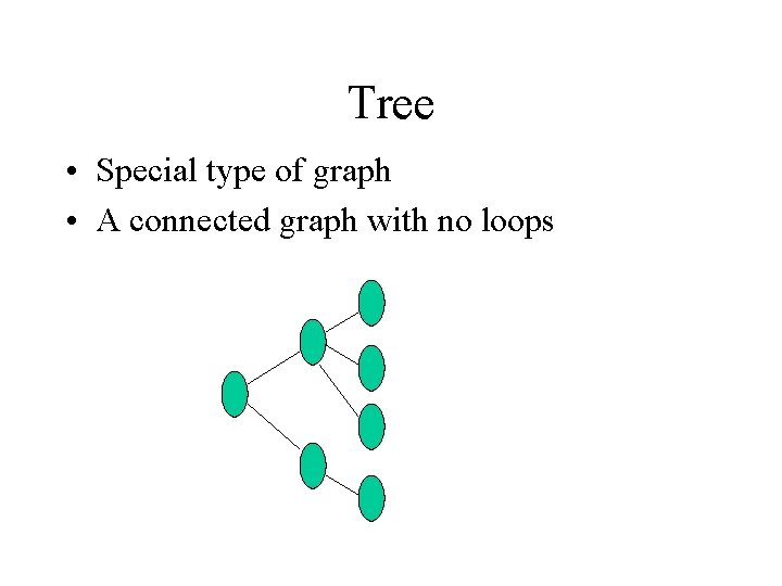
Tree • Special type of graph • A connected graph with no loops

Problem solving with graphs • Many problems can be formulated as graph problems – Find a path from vertex a to vertex b – Find the shortest path from a to b – Find the lowest cost path from a to b – For example Internet router systems • Find a path from a to b that has low cost and can satisfy certain quality of service constraints

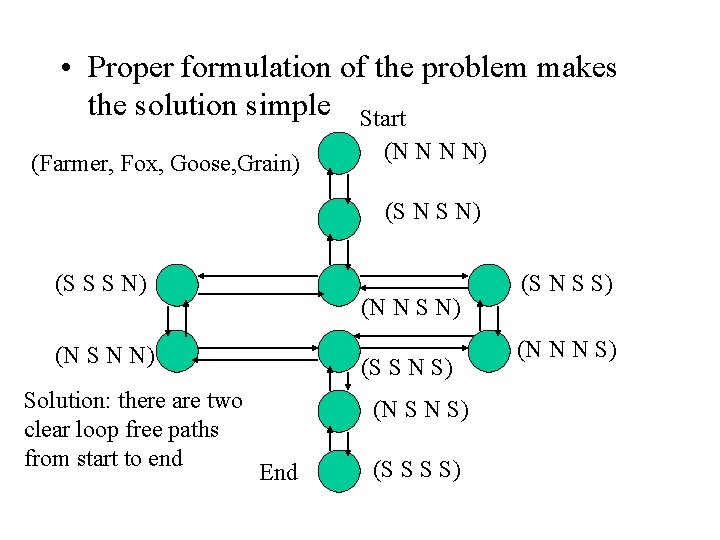
Example The farmer and his goose • Classic puzzle – Farmer, Fox, Goose, Grain and River with a rowboat – Farmer can’t leave Fox alone with Goose, or Goose alone with Grain – Initially all on north side of river. – Problem • Discover how to get to the south side

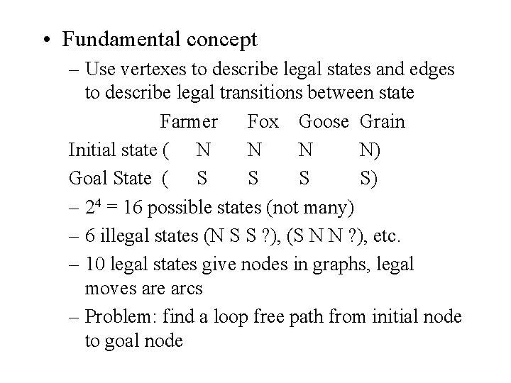
• Fundamental concept – Use vertexes to describe legal states and edges to describe legal transitions between state Farmer Fox Goose Grain Initial state ( N N) Goal State ( S S) – 24 = 16 possible states (not many) – 6 illegal states (N S S ? ), (S N N ? ), etc. – 10 legal states give nodes in graphs, legal moves are arcs – Problem: find a loop free path from initial node to goal node

• Proper formulation of the problem makes the solution simple Start (Farmer, Fox, Goose, Grain) (N N N N) (S N S N) (S S S N) (N N S N) (N S N N) Solution: there are two clear loop free paths from start to end (S S N S) (N S N S) End (S S S S) (S N S S) (N N N S)

Graph representations • We consider four – Matrix representation – Array/adjacency list for digraph – Pure graph – Edge list

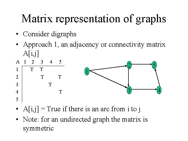
Matrix representation of graphs • Consider digraphs • Approach 1, an adjacency or connectivity matrix A[i, j] A 1 2 1 T 2 3 4 5 3 T T 4 5 T T T 1 2 3 • A[i, j] = True if there is an arc from i to j • Note: for an undirected graph the matrix is symmetric 5 4

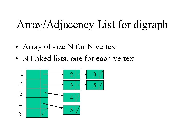
Array/Adjacency List for digraph • Array of size N for N vertex • N linked lists, one for each vertex 1 2 3 3 5 4 5

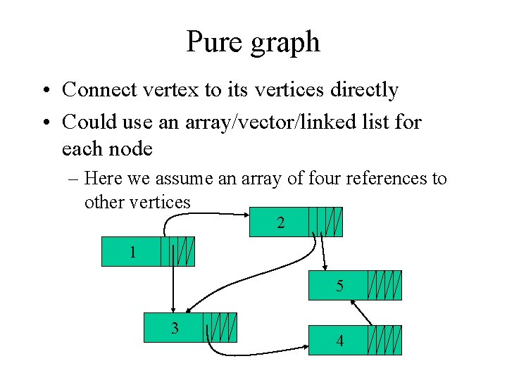
Pure graph • Connect vertex to its vertices directly • Could use an array/vector/linked list for each node – Here we assume an array of four references to other vertices 2 1 5 3 4

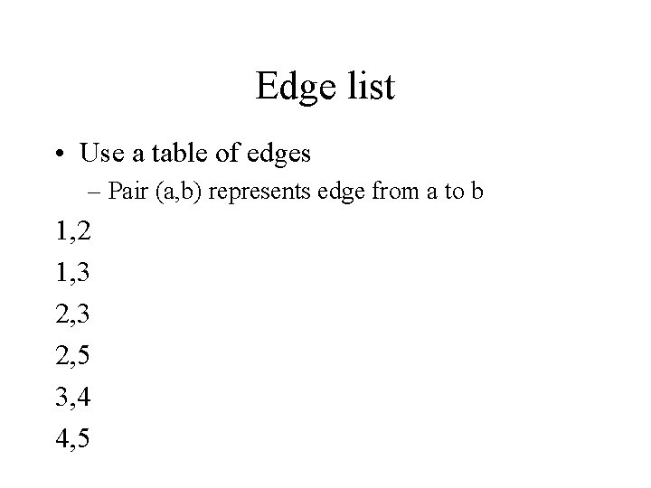
Edge list • Use a table of edges – Pair (a, b) represents edge from a to b 1, 2 1, 3 2, 5 3, 4 4, 5

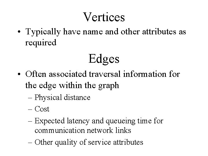
Vertices • Typically have name and other attributes as required Edges • Often associated traversal information for the edge within the graph – Physical distance – Cost – Expected latency and queueing time for communication network links – Other quality of service attributes

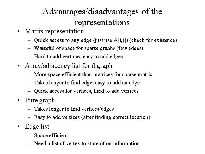
Advantages/disadvantages of the representations • Matrix representation – Quick access to any edge (just use A[i, j]) (check for existence) – Wasteful of space for sparse graphs (few edges) – Hard to add vertices, easy to add edges • Array/adjacency list for digraph – More space efficient than matrices for sparse matrix – Takes longer to find edge, easy to add an edge – Quick access for vertices, hard to add vertices • Pure graph – Takes longer to find vertices/edges – Easy to add vertices (after finding correct location) • Edge list – Space efficient – Need a list of vertex to store other information

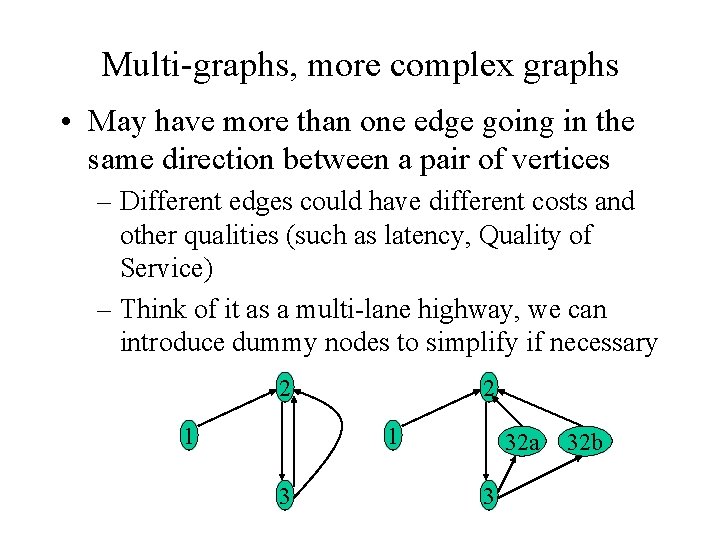
Multi-graphs, more complex graphs • May have more than one edge going in the same direction between a pair of vertices – Different edges could have different costs and other qualities (such as latency, Quality of Service) – Think of it as a multi-lane highway, we can introduce dummy nodes to simplify if necessary 2 1 3 32 a 3 32 b

ADT Graph • • • Create Read Write Iterator (graph traversal) Generate a path between two vertices Generate a least cost path between two vertices

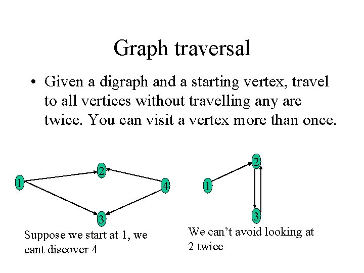
Graph traversal • Given a digraph and a starting vertex, travel to all vertices without travelling any arc twice. You can visit a vertex more than once. 1 2 2 4 3 Suppose we start at 1, we cant discover 4 1 3 We can’t avoid looking at 2 twice

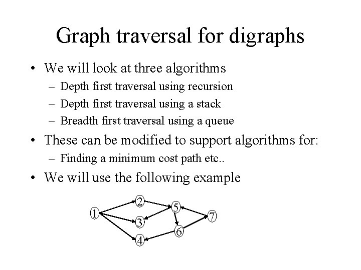
Graph traversal for digraphs • We will look at three algorithms – Depth first traversal using recursion – Depth first traversal using a stack – Breadth first traversal using a queue • These can be modified to support algorithms for: – Finding a minimum cost path etc. . • We will use the following example 1 2 3 4 5 6 7

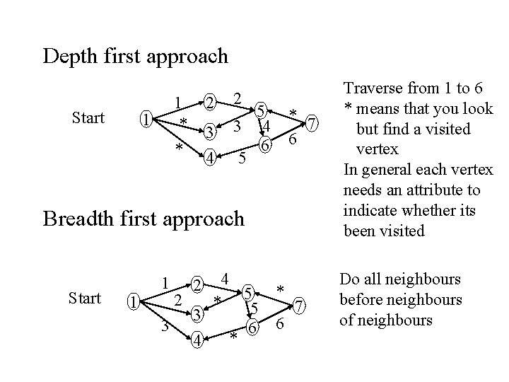
Depth first approach Start 2 1 * * 1 3 4 2 5 3 4 6 5 * 7 6 Breadth first approach Start 4 2 * 55 3 3 6 * 4 1 1 2 * 6 7 Traverse from 1 to 6 * means that you look but find a visited vertex In general each vertex needs an attribute to indicate whether its been visited Do all neighbours before neighbours of neighbours

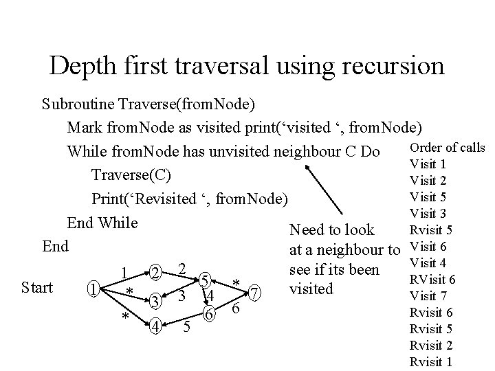
Depth first traversal using recursion Subroutine Traverse(from. Node) Mark from. Node as visited print(‘visited ‘, from. Node) Order of calls While from. Node has unvisited neighbour C Do Visit 1 Traverse(C) Visit 2 Visit 5 Print(‘Revisited ‘, from. Node) Visit 3 End While Rvisit 5 Need to look End at a neighbour to Visit 6 Visit 4 2 see if its been 1 2 RVisit 6 5 * Start visited 1 * 3 3 4 7 Visit 7 6 Rvisit 6 * 4 5 6 Rvisit 5 Rvisit 2 Rvisit 1

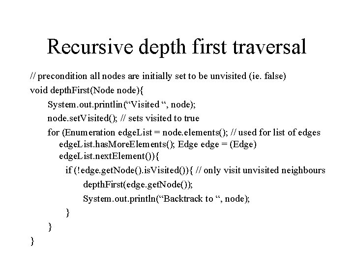
Recursive depth first traversal // precondition all nodes are initially set to be unvisited (ie. false) void depth. First(Node node){ System. out. printlin(“Visited “, node); node. set. Visited(); // sets visited to true for (Enumeration edge. List = node. elements(); // used for list of edges edge. List. has. More. Elements(); Edge edge = (Edge) edge. List. next. Element()){ if (!edge. get. Node(). is. Visited()){ // only visit unvisited neighbours depth. First(edge. get. Node()); System. out. println(“Backtrack to “, node); } } }

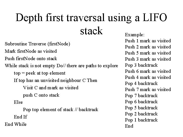
Depth first traversal using a LIFO stack Example: Subroutine Traverse (first. Node) Mark first. Node as visited Push first. Node onto stack While stack is not empty Do// there are paths to explore top = peek at top element If top has an unvisited neighbour C Then Visit C and mark as visited push C onto stack Else Pop top element of stack // backtrack End If End While Push 1 mark as visited Push 2 mark as visited Push 5 mark as visited Push 3 mark as visited Pop 3 backtrack Push 6 mark as visited Push 4 mark as visited Pop 4 backtrack Push 7 mark as visited Pop 7 backtrack Pop 6 backtrack Pop 5 backtrack Pop 2 backtrack Pop 1 backtrack End

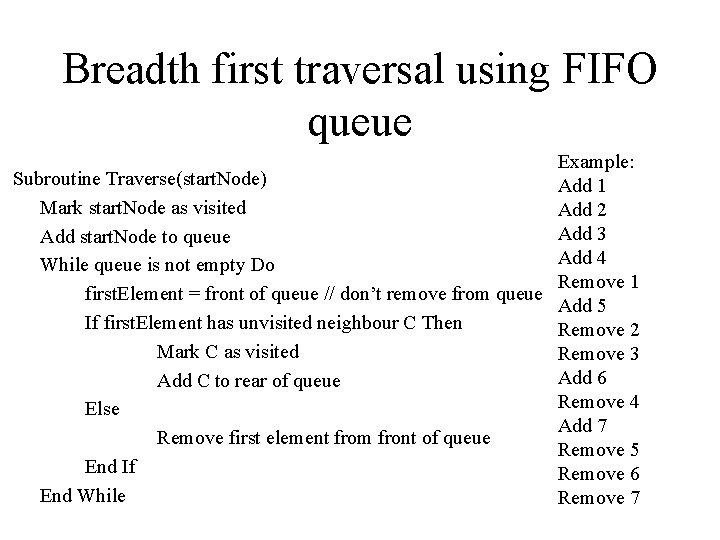
Breadth first traversal using FIFO queue Example: Subroutine Traverse(start. Node) Add 1 Mark start. Node as visited Add 2 Add 3 Add start. Node to queue Add 4 While queue is not empty Do Remove 1 first. Element = front of queue // don’t remove from queue Add 5 If first. Element has unvisited neighbour C Then Remove 2 Mark C as visited Remove 3 Add 6 Add C to rear of queue Remove 4 Else Add 7 Remove first element from front of queue Remove 5 End If Remove 6 End While Remove 7

Finding a path from vertex a to vertex b • Can modify the a depth first traversal to stop once b is found • The path is stored on: • The program stack via local variables created for a recursive call for the recursive version • The stack for the non-recursive version

Finding the shortest path in a directed graph • Dijkstra’s Algorithm for shortest or least costly path between two vertices in a graph • Approach – Find the shortest path from one vertex (the source) to all other vertices – Referred to as a greedy algorithm

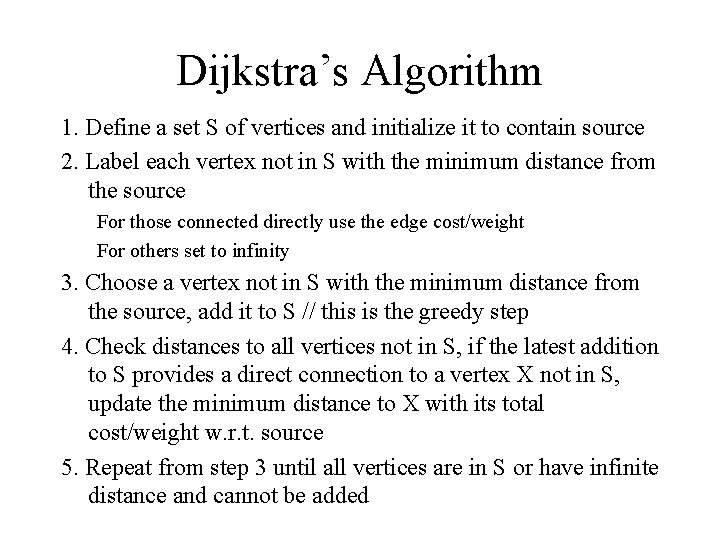
Dijkstra’s Algorithm 1. Define a set S of vertices and initialize it to contain source 2. Label each vertex not in S with the minimum distance from the source For those connected directly use the edge cost/weight For others set to infinity 3. Choose a vertex not in S with the minimum distance from the source, add it to S // this is the greedy step 4. Check distances to all vertices not in S, if the latest addition to S provides a direct connection to a vertex X not in S, update the minimum distance to X with its total cost/weight w. r. t. source 5. Repeat from step 3 until all vertices are in S or have infinite distance and cannot be added

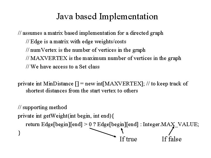
Java based Implementation // assumes a matrix based implementation for a directed graph // Edge is a matrix with edge weights/costs // num. Vertex is the number of vertices in the graph // MAXVERTEX is the maximum number of vertices in the graph // We have access to a Set class private int Min. Distance [] = new int[MAXVERTEX]; // to keep track of shortest distances from the start vertex to others // supporting method private int get. Weight(int begin, int end){ return Edge[begin][end] > 0 ? Edge[begin][end] : Integer. MAX_VALUE; } If true If false

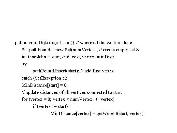
public void Dijkstra(int start){ // where all the work is done Set path. Found = new Set(num. Vertex); // create empty set S int temp. Min = start, end, cost, vertex, min. Dist; try path. Found. Insert(start); // add first vertex catch (Set. Exception e); Min. Distance[start] = 0; // update distances of all vertices connected to start for (vertex = 0; vertex < num. Vertex; ++vertex) if (vertex != start) Min. Distance[vertex] = get. Weight(start, vertex);

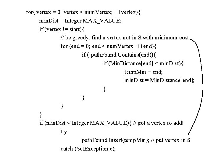
for( vertex = 0; vertex < num. Vertex; ++vertex){ min. Dist = Integer. MAX_VALUE; if (vertex != start){ // be greedy, find a vertex not in S with minimum cost for (end = 0; end < num. Vertex; ++end){ if (!path. Found. Contains(end)){ if (Min. Distance[end] < min. Dist){ temp. Min = end; min. Dist = Min. Distance[end]; } } if (min. Dist < Integer. MAX_VALUE){ // got a vertex to add! try path. Found. Insert(temp. Min); // put vertex in S catch (Set. Exception e);

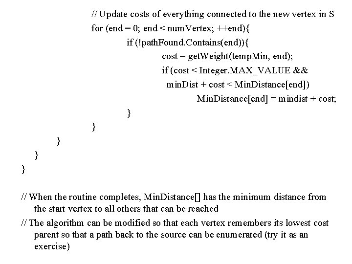
// Update costs of everything connected to the new vertex in S for (end = 0; end < num. Vertex; ++end){ if (!path. Found. Contains(end)){ cost = get. Weight(temp. Min, end); if (cost < Integer. MAX_VALUE && min. Dist + cost < Min. Distance[end]) Min. Distance[end] = mindist + cost; } } } // When the routine completes, Min. Distance[] has the minimum distance from the start vertex to all others that can be reached // The algorithm can be modified so that each vertex remembers its lowest cost parent so that a path back to the source can be enumerated (try it as an exercise)