Forecasting for Operations Everette S Gardner Jr 1

Forecasting for Operations Everette S. Gardner, Jr. 1

Forecasting for operations q Research themes q The damped trend q Case studies 1. Supply chain costs: Specialty chemicals 2. Manufacturing inventory investment: Snack foods 3. Purchasing workload: Water treatment systems q Consequences of forecast errors q How to evaluate forecast performance 2

Research themes q Intermittent demand q Distribution inventory management q Biased forecasting q Bullwhip effect q Sensitivity of costs to forecast errors 3

Intermittent demand q Empirical research is mixed - not clear that intermittent methods can beat SES q No underlying model exists for the Croston method or any of its variants (Shenstone & Hyndman, IJF, 2005) q Why not remove zeroes by aggregation? (Nikolopoulos et al. , JORS, 2011) 4

Distribution inventory management q The damped trend gives better inventory performance than other exponential smoothing methods (Gardner, MS, 1990) q Marginal improvements in forecast accuracy produce much larger improvements in inventory costs (Syntetos et al. , IJF, 2010) 5

Biased forecasting q Effects (Sanders & Graman, Omega, 2009) q Costs are more sensitive to bias than variance q Over-forecasting produces lower costs than unbiased forecasting in an MRP environment q Objections q Conclusions depend on assumptions q Safety stock is always a better option than adding bias to the forecasts 6

The bullwhip effect q Definition q Tendency of demand variability to increase as one moves up a supply chain q Caused by lead times and forecast errors q Is the bullwhip effect inevitable? q Yes – But it can be reduced with centralized demand information (Chen et al. , MS, 2000) q No – Bullwhip effect is due to poor research design (Fildes & Kingsman, JORS, 2010) 7

Sensitivity of costs to forecast error q Fildes and Kingsman (JORS, 2011) q Research design q q Conclusions q q 8 MRP simulation Distinguishes between noise and specification error Demand processes are experimental factors Cost increases exponentially with demand uncertainty Cost benefits of improved forecasting are greater than the effects of choosing inventory decision rules

Performance of the damped trend q “The damped trend is a well established forecasting method that should improve accuracy in practical applications. ” (Armstrong, IJF, 2006) q “The damped trend can reasonably claim to be a benchmark forecasting method for all others to beat. ” (Fildes et al. , JORS, 2008) 9

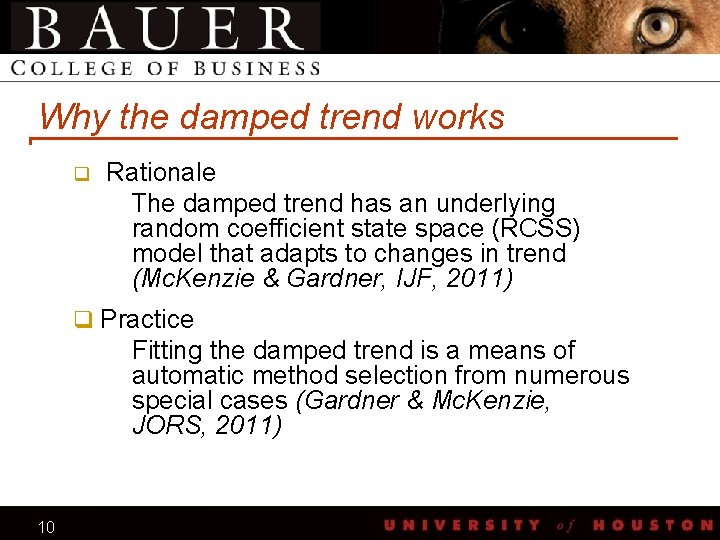
Why the damped trend works q Rationale The damped trend has an underlying random coefficient state space (RCSS) model that adapts to changes in trend (Mc. Kenzie & Gardner, IJF, 2011) q Practice Fitting the damped trend is a means of automatic method selection from numerous special cases (Gardner & Mc. Kenzie, JORS, 2011) 10

SSOE state space models q q q 11 {At} are i. i. d. binary random variates White noise innovation processes ε and are different Parameters h and h* are related but usually different

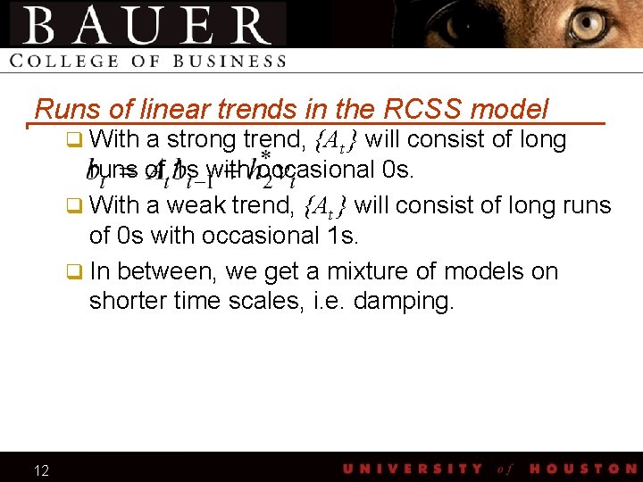
Runs of linear trends in the RCSS model q With a strong trend, {At } will consist of long runs of 1 s with occasional 0 s. q With a weak trend, {At } will consist of long runs of 0 s with occasional 1 s. q In between, we get a mixture of models on shorter time scales, i. e. damping. 12

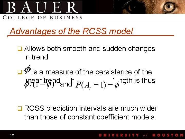
Advantages of the RCSS model q Allows both smooth and sudden changes in trend. q is a measure of the persistence of the linear trend. and The mean run length is thus q RCSS prediction intervals are much wider than those of constant coefficient models. 13

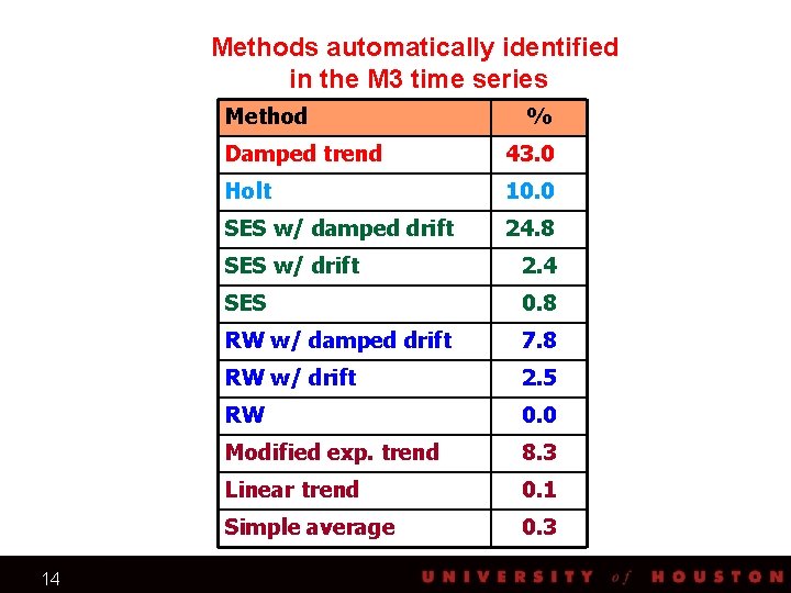
Methods automatically identified in the M 3 time series Method 14 % Damped trend 43. 0 Holt 10. 0 SES w/ damped drift 24. 8 SES w/ drift 2. 4 SES 0. 8 RW w/ damped drift 7. 8 RW w/ drift 2. 5 RW 0. 0 Modified exp. trend 8. 3 Linear trend 0. 1 Simple average 0. 3

Case 1: Chemicals supply chain q Scope q 4 plants: N. and S. America, Europe, Asia q 10 component chemicals, 25 products q 400 customers, 250, 000 tons of annual production q Production and transportation plans based on q Damped trend q Optimization q Simulation 15

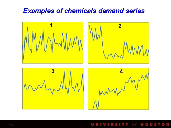
Examples of chemicals demand series 1 3 16 2 4

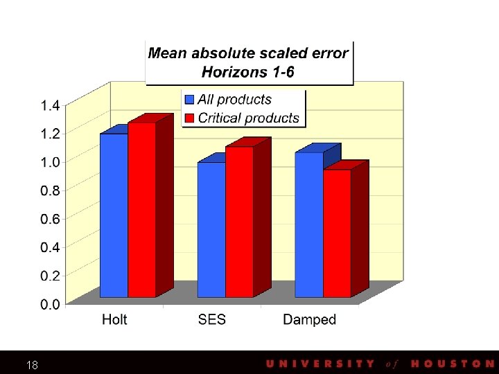
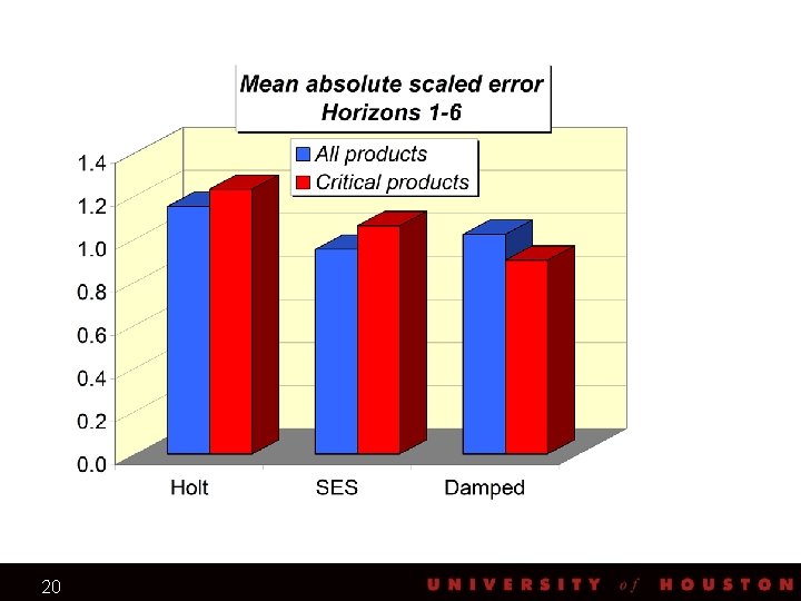
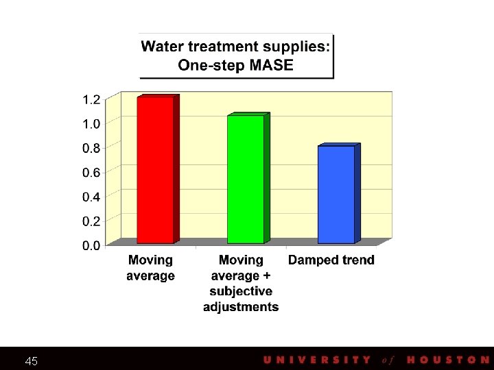
Scaled errors q Average forecast error measures are misleading q Drastic changes in scale q Some observations near zero q Alternative - Scaled errors (Hyndman & Koehler, 2006) q q 17 Based on in-sample, one-step errors from the naïve method If scaled error is less than 1, we beat the naïve method

18

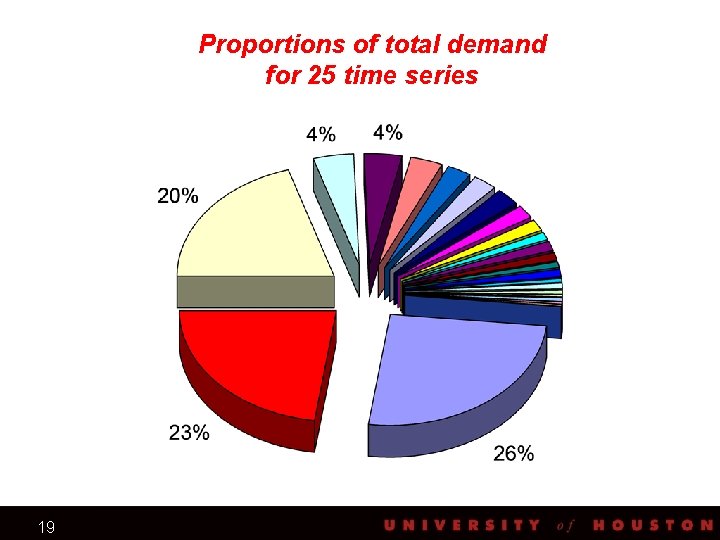
Proportions of total demand for 25 time series 19

20

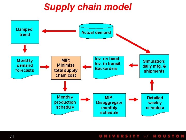
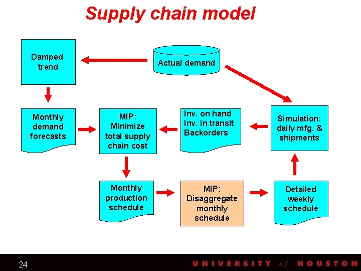
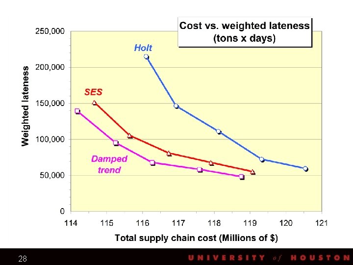
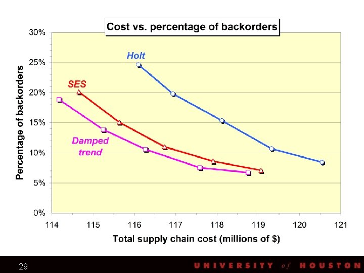
Supply chain model Damped trend Monthly demand forecasts Actual demand MIP: Minimize total supply chain cost Monthly production schedule 21 Inv. on hand Inv. in transit Backorders MIP: Disaggregate monthly schedule Simulation: daily mfg. & shipments Detailed weekly schedule

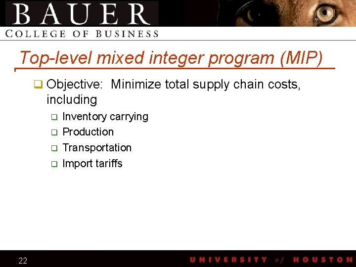
Top-level mixed integer program (MIP) q Objective: Minimize total supply chain costs, including q q 22 Inventory carrying Production Transportation Import tariffs

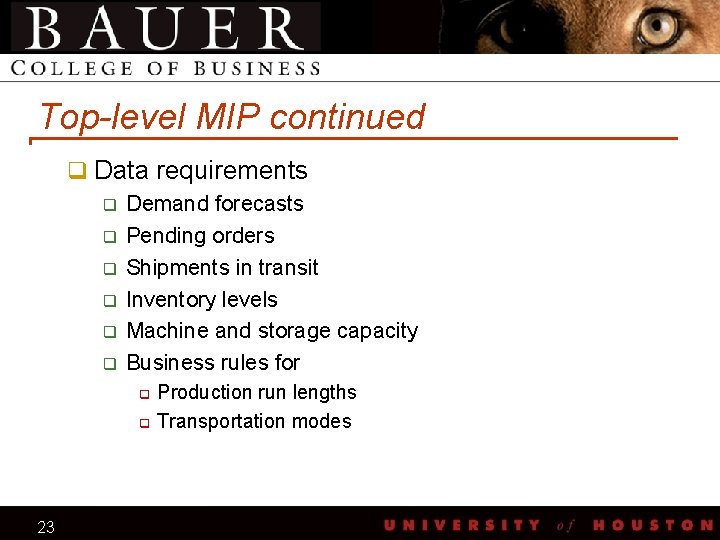
Top-level MIP continued q Data requirements q Demand forecasts q Pending orders q Shipments in transit q Inventory levels q Machine and storage capacity q Business rules for q q 23 Production run lengths Transportation modes

Supply chain model Damped trend Monthly demand forecasts Actual demand MIP: Minimize total supply chain cost Monthly production schedule 24 Inv. on hand Inv. in transit Backorders MIP: Disaggregate monthly schedule Simulation: daily mfg. & shipments Detailed weekly schedule

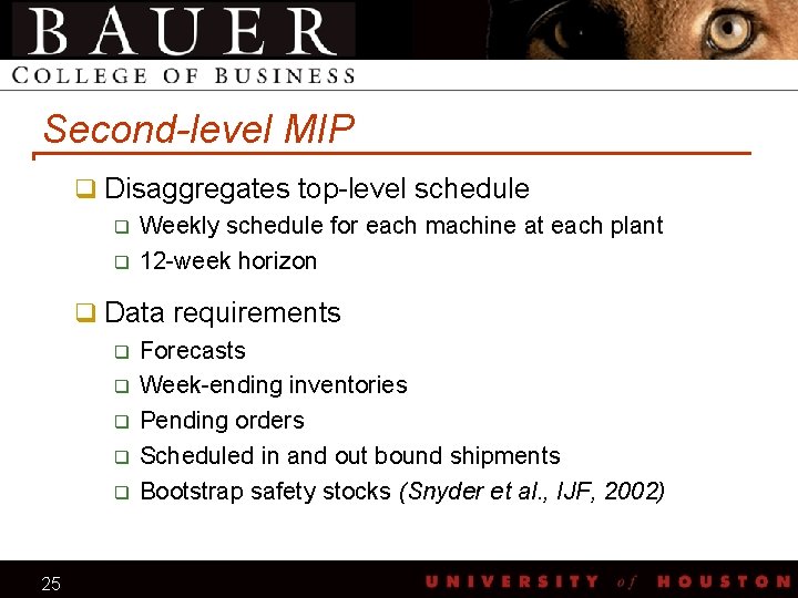
Second-level MIP q Disaggregates top-level schedule q Weekly schedule for each machine at each plant q 12 -week horizon q Data requirements q Forecasts q Week-ending inventories q Pending orders q Scheduled in and out bound shipments q Bootstrap safety stocks (Snyder et al. , IJF, 2002) 25

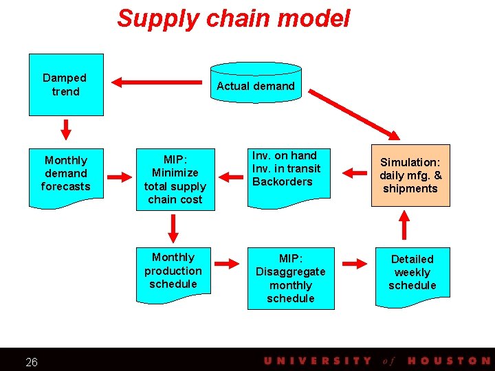
Supply chain model Damped trend Monthly demand forecasts Actual demand MIP: Minimize total supply chain cost Monthly production schedule 26 Inv. on hand Inv. in transit Backorders MIP: Disaggregate monthly schedule Simulation: daily mfg. & shipments Detailed weekly schedule

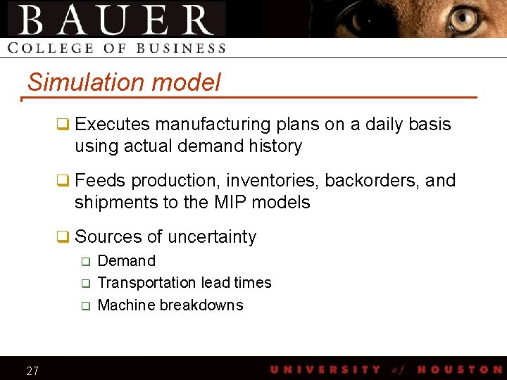
Simulation model q Executes manufacturing plans on a daily basis using actual demand history q Feeds production, inventories, backorders, and shipments to the MIP models q Sources of uncertainty q Demand q Transportation lead times q Machine breakdowns 27

28

29

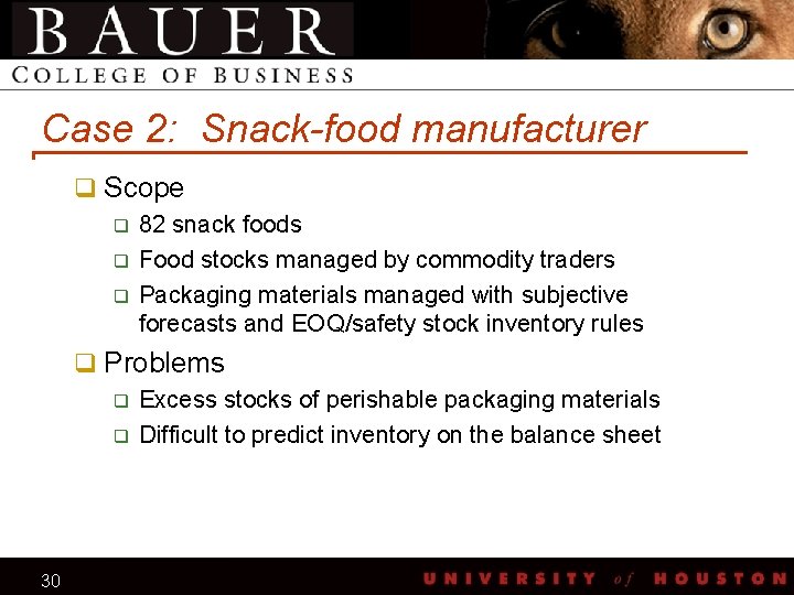
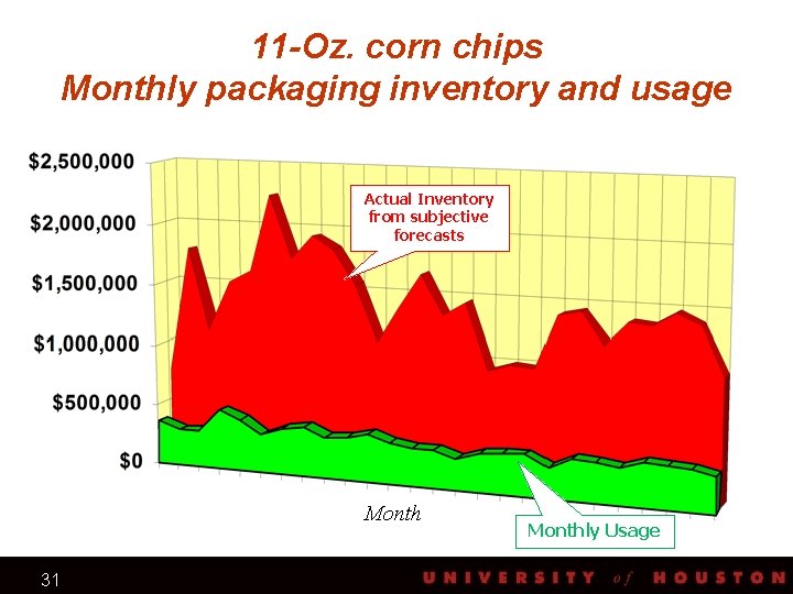
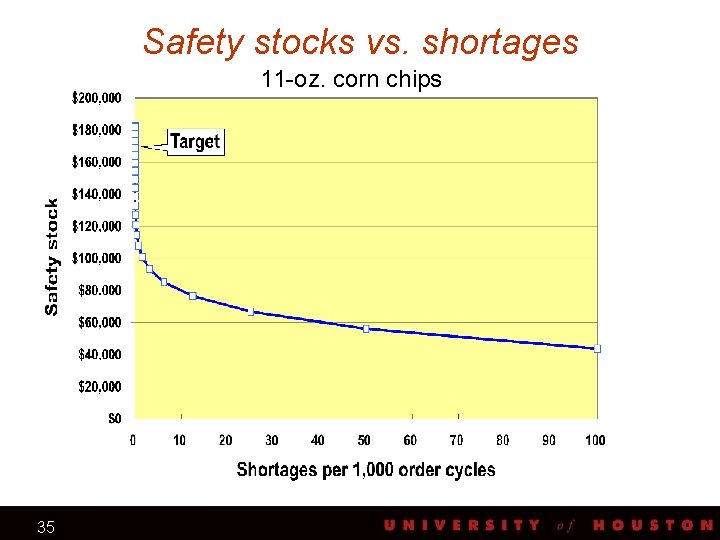
Case 2: Snack-food manufacturer q Scope q 82 snack foods q Food stocks managed by commodity traders q Packaging materials managed with subjective forecasts and EOQ/safety stock inventory rules q Problems q Excess stocks of perishable packaging materials q Difficult to predict inventory on the balance sheet 30

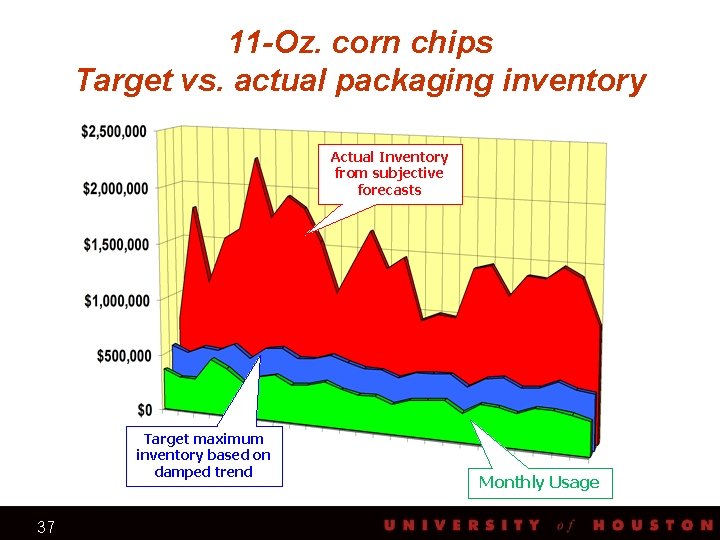
11 -Oz. corn chips Monthly packaging inventory and usage Actual Inventory from subjective forecasts Month 31 Monthly Usage

Snack-food manufacturer q Solution q Automatic forecasting with the damped trend q Retain EOQ/safety stock inventory rules 32

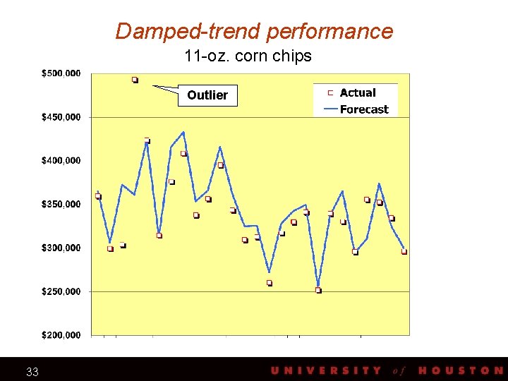
Damped-trend performance 11 -oz. corn chips Outlier 33

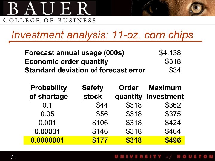
Investment analysis: 11 -oz. corn chips 34

Safety stocks vs. shortages 11 -oz. corn chips 35

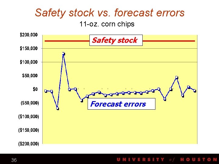
Safety stock vs. forecast errors 11 -oz. corn chips Safety stock Forecast errors 36

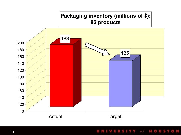
11 -Oz. corn chips Target vs. actual packaging inventory Actual Inventory from subjective Actual Inventory forecasts from subjective forecasts Target maximum inventory based on damped trend 37 Monthly Usage

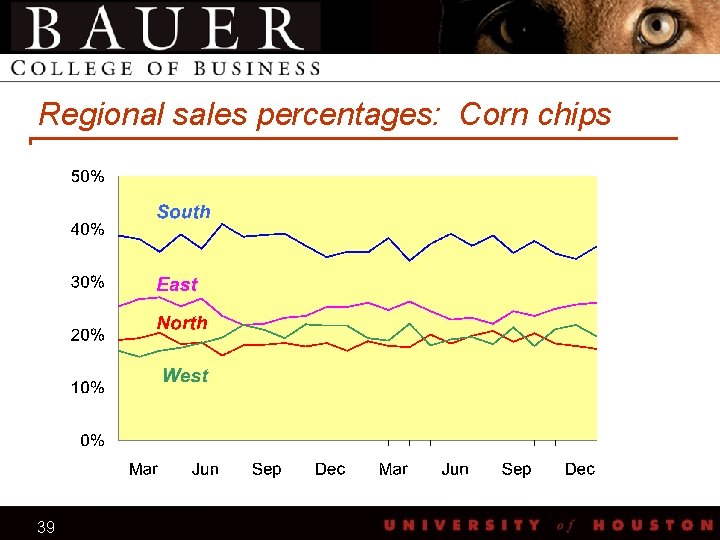
Forecasting regional demand q Forecast total unit demand with the damped trend q Forecast regional percentages with simple exponential smoothing 38

Regional sales percentages: Corn chips 39

40

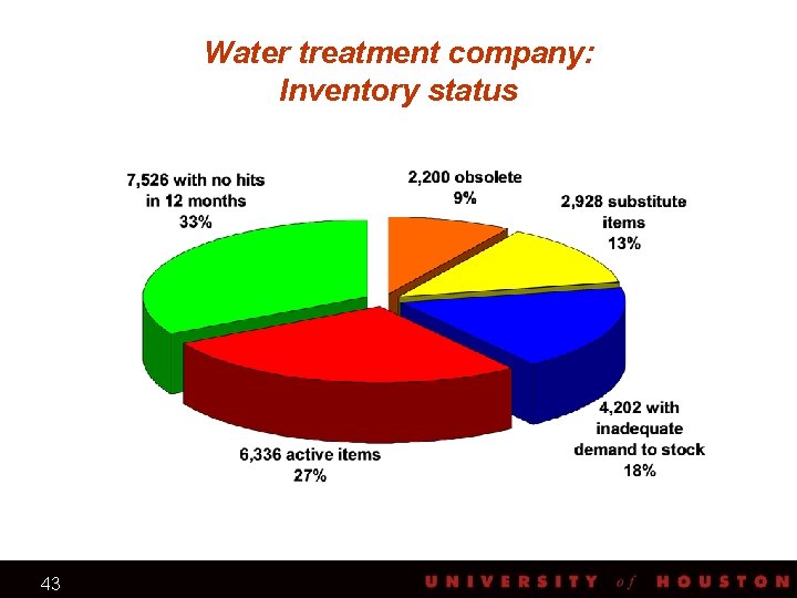
Case 3: Water treatment company q Scope q Assembly of systems and distribution of supplies q Annual sales = $16 million q Inventory = $6 million (23, 000 SKUs) q Inventory system q Reorder monthly to maintain 3 months of stock q Numerous subjective adjustments q Forecasting system q 6 -month weighted moving average q Numerous subjective adjustments 41

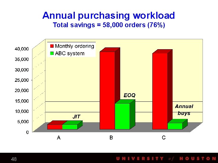
Problems q Forecasts vs. reality q Annual forecasts on stock records = $29 million q Annual sales = $16 million q Purchasing workload q 76, 000 purchase orders per year q Messy stock records 42 q Dead stock q Substitute items not linked to primary items

Water treatment company: Inventory status 43

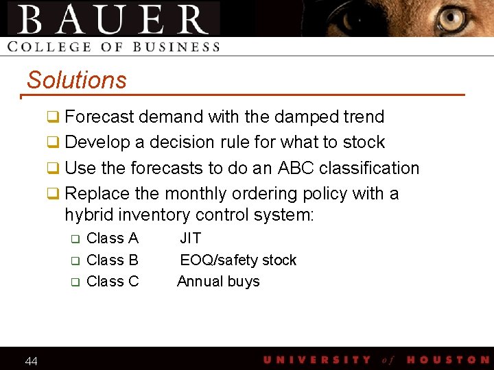
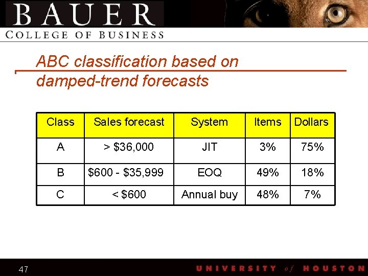
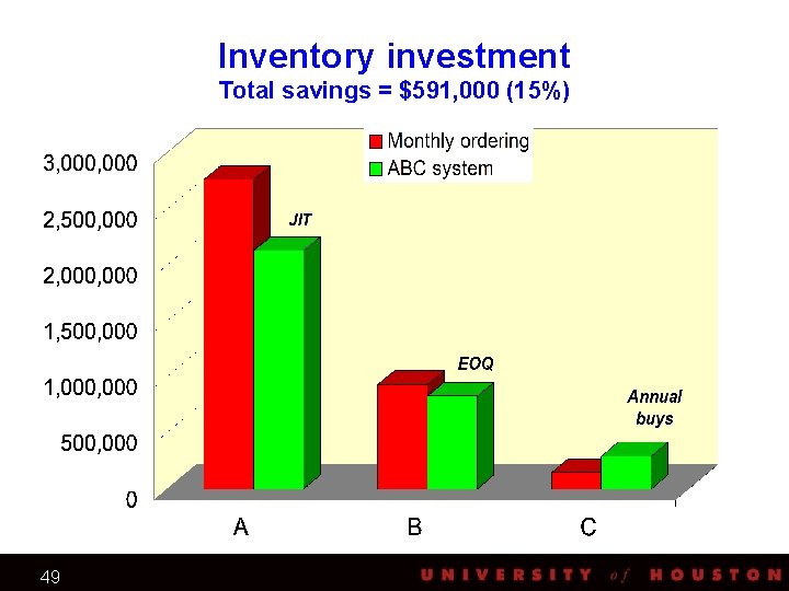
Solutions q Forecast demand with the damped trend q Develop a decision rule for what to stock q Use the forecasts to do an ABC classification q Replace the monthly ordering policy with a hybrid inventory control system: q q q 44 Class A Class B Class C JIT EOQ/safety stock Annual buys

45

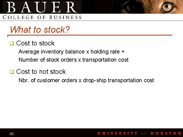
What to stock? q Cost to stock Average inventory balance x holding rate + Number of stock orders x transportation cost q Cost to not stock Nbr. of customer orders x drop-ship transportation cost 46

ABC classification based on damped-trend forecasts 47 Class Sales forecast System Items Dollars A > $36, 000 JIT 3% 75% B $600 - $35, 999 EOQ 49% 18% C < $600 Annual buy 48% 7%

Annual purchasing workload Total savings = 58, 000 orders (76%) EOQ JIT 48

Inventory investment Total savings = $591, 000 (15%) EOQ JIT 49

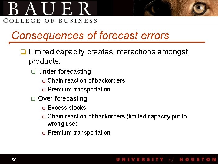
Consequences of forecast errors q Limited capacity creates interactions amongst products: q Under-forecasting q q q Over-forecasting q q q 50 Chain reaction of backorders Premium transportation Excess stocks Chain reaction of backorders (limited capacity put to wrong use) Premium transportation

Consequences of forecast errors (cont. ) q Errors often reverse themselves before system has fully responded to q q 51 Backorders, or Excess stocks

How to evaluate forecast performance q Operational measures q Backorder delay time q Percent of time in stock q Percent of orders filled immediately q Number of purchase orders or production setups q Financial measures q Manufacturing, distribution, and supply chain costs q Value of backorders q Inventory investment on the balance sheet 52

Future research q Research is needed: q In real operating systems Gardner & Makridakis (IJF, 1988) q On the benefits of improved forecasting Fildes & Kingsman (JORS, 2010) q On the relationship between forecast accuracy and operational performance Syntetos et al. (IJF, 2010) 53

Presentation and papers available at www. bauer. uh. edu/gardner 54