Demand Forecasting Production and Operations Management Judit UzonyiKecsks

Demand Forecasting Production and Operations Management Judit Uzonyi-Kecskés Ph. D. Student Department of Management and Corporate Economics Budapest University of Technology and Economics uzonyi-kecskes@mvt. bme. hu

Topics • Introduction • Forecasting methods • Forecasting stationary series – Moving average (with example) – Simple exponential smoothing (with example) • Trend based forecasting methods – Double exponential smoothing (with example) • Evaluating forecasts – Analyzing the size of errors (with example) – Analyzing the validity of the forecasting model (with example)

Forecasting • • Find balance of supply and demand Predicting the future Production and service area Application of forecasting results: – Capacity planning – Production scheduling – Inventory control – Materials requirement planning

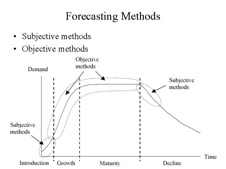
Forecasting Methods • Subjective methods • Objective methods

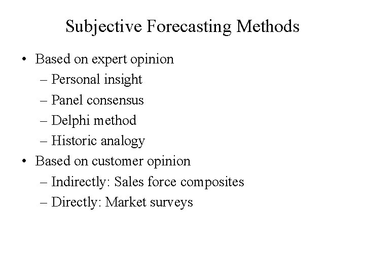
Subjective Forecasting Methods • Based on expert opinion – Personal insight – Panel consensus – Delphi method – Historic analogy • Based on customer opinion – Indirectly: Sales force composites – Directly: Market surveys

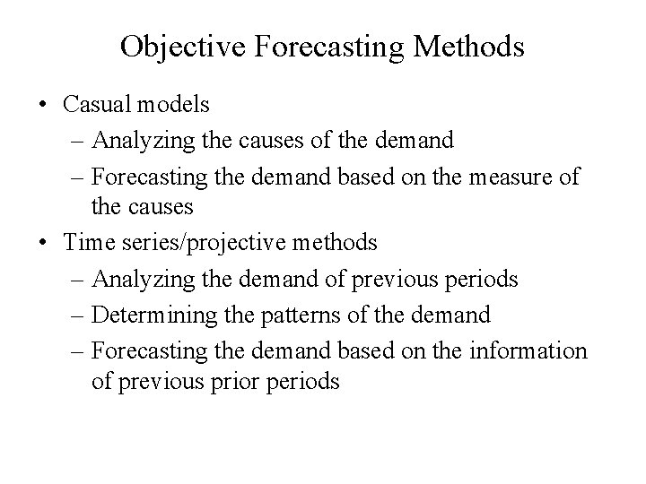
Objective Forecasting Methods • Casual models – Analyzing the causes of the demand – Forecasting the demand based on the measure of the causes • Time series/projective methods – Analyzing the demand of previous periods – Determining the patterns of the demand – Forecasting the demand based on the information of previous prior periods

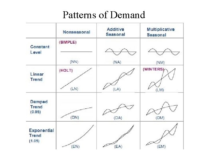
Patterns of Demand

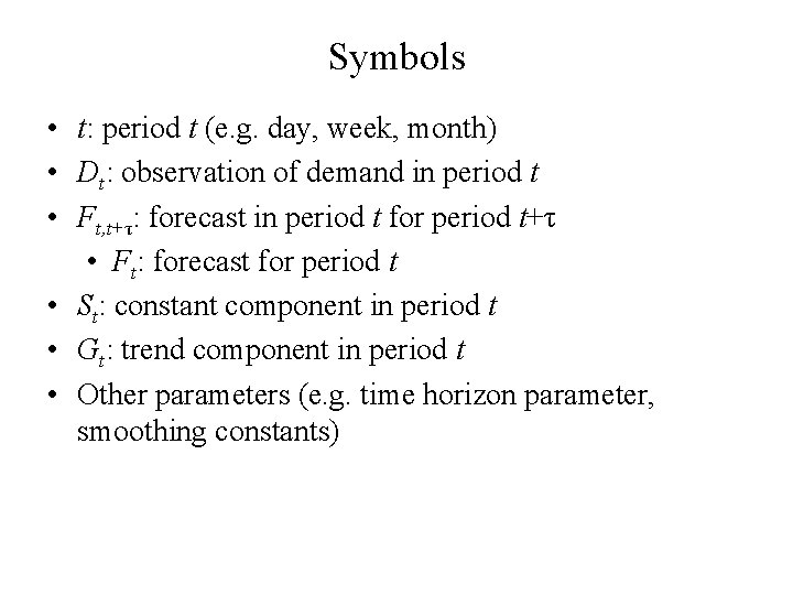
Symbols • t: period t (e. g. day, week, month) • Dt: observation of demand in period t • Ft, t+τ: forecast in period t for period t+τ • Ft: forecast for period t • St: constant component in period t • Gt: trend component in period t • Other parameters (e. g. time horizon parameter, smoothing constants)

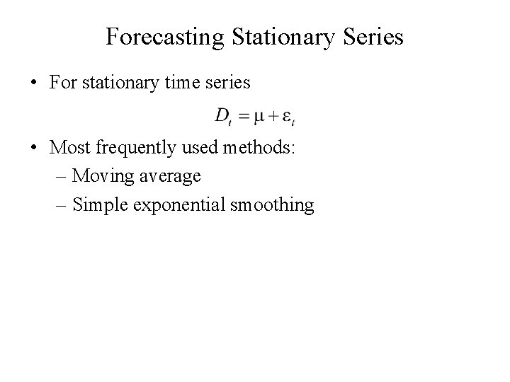
Forecasting Stationary Series • For stationary time series • Most frequently used methods: – Moving average – Simple exponential smoothing

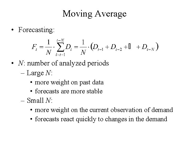
Moving Average • Forecasting: • N: number of analyzed periods – Large N: • more weight on past data • forecasts are more stable – Small N: • more weight on the current observation of demand • forecasts react quickly to changes in the demand

Example In a car factory the management observed that the demand for the factory’s car is nearly constant. Therefore they forecast the demand with the help of moving average based on the demand information of the last 2 months.

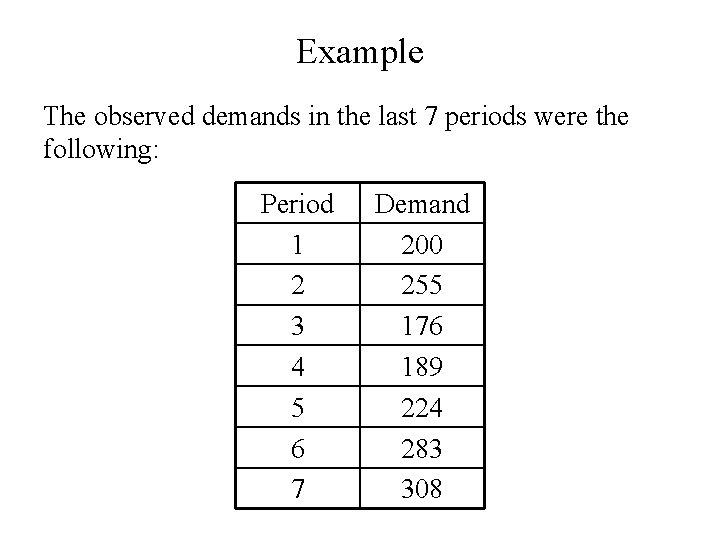
Example The observed demands in the last 7 periods were the following: Period 1 2 3 4 5 6 7 Demand 200 255 176 189 224 283 308

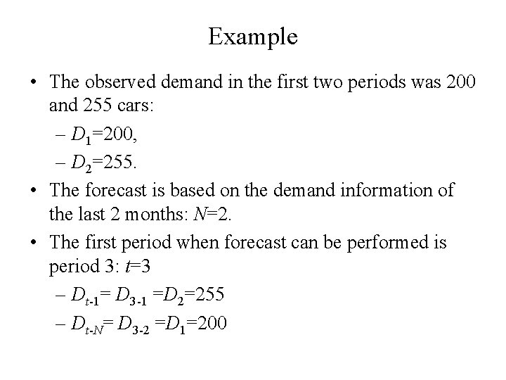
Example • The observed demand in the first two periods was 200 and 255 cars: – D 1=200, – D 2=255. • The forecast is based on the demand information of the last 2 months: N=2. • The first period when forecast can be performed is period 3: t=3 – Dt-1= D 3 -1 =D 2=255 – Dt-N= D 3 -2 =D 1=200

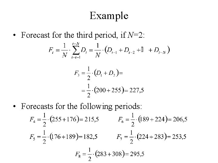
Example • Forecast for the third period, if N=2: • Forecasts for the following periods:

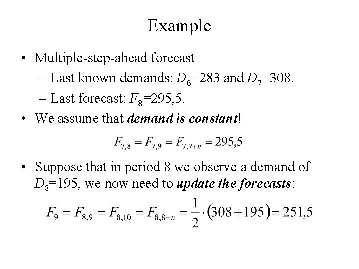
Example • Multiple-step-ahead forecast – Last known demands: D 6=283 and D 7=308. – Last forecast: F 8=295, 5. • We assume that demand is constant! • Suppose that in period 8 we observe a demand of D 8=195, we now need to update the forecasts:

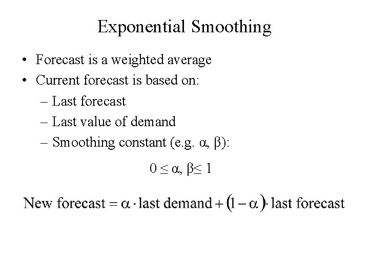
Exponential Smoothing • Forecast is a weighted average • Current forecast is based on: – Last forecast – Last value of demand – Smoothing constant (e. g. α, β): 0 ≤ α, β≤ 1

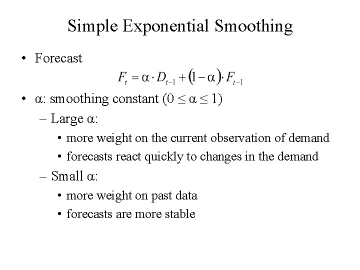
Simple Exponential Smoothing • Forecast • α: smoothing constant (0 ≤ α ≤ 1) – Large α: • more weight on the current observation of demand • forecasts react quickly to changes in the demand – Small α: • more weight on past data • forecasts are more stable

Example In a car factory the management observed that the demand for the factory’s car is nearly constant. Therefore they forecast the demand with the help of simple exponential smoothing, and they use α=0. 1 value as smoothing constant. The forecast for the first period was 250 cars.

Example The observed demands in the last 7 periods were the following: Period 1 2 3 4 5 6 7 Demand 200 250 176 189 224 283 308

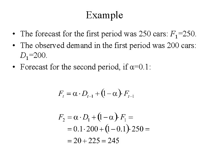
Example • The forecast for the first period was 250 cars: F 1=250. • The observed demand in the first period was 200 cars: D 1=200. • Forecast for the second period, if α=0. 1:

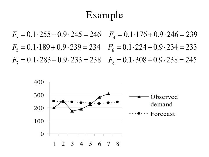
Example

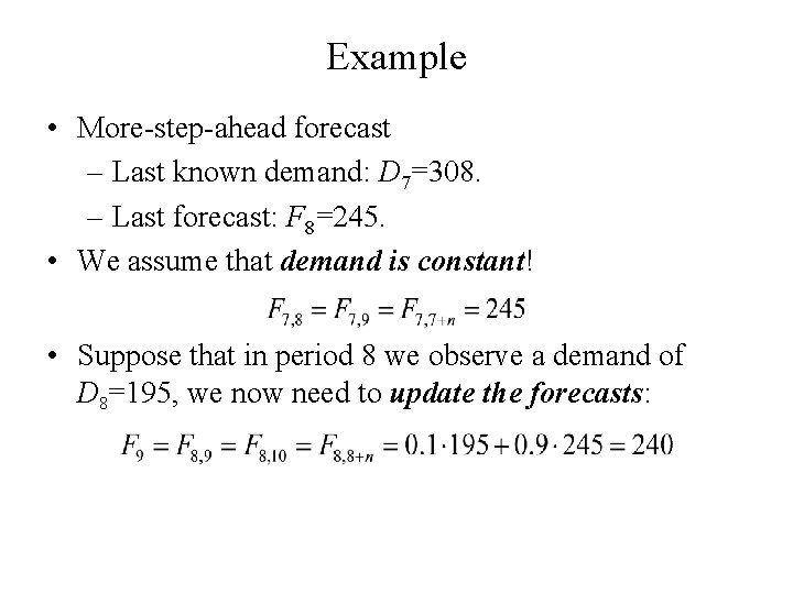
Example • More-step-ahead forecast – Last known demand: D 7=308. – Last forecast: F 8=245. • We assume that demand is constant! • Suppose that in period 8 we observe a demand of D 8=195, we now need to update the forecasts:

Comparison of the Two Methods • Similarities – Both assume that demand is stationary – Both use a single parameter (N or α) • Differences – Number of directly used demand data – Number and weights of indirectly used demand data

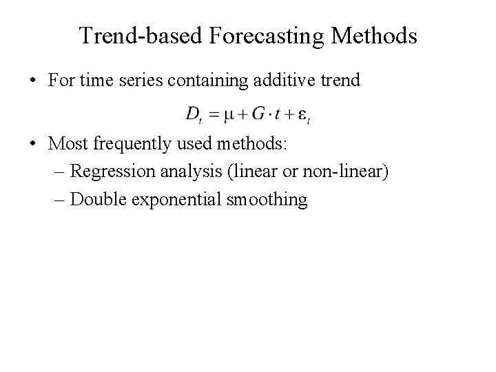
Trend-based Forecasting Methods • For time series containing additive trend • Most frequently used methods: – Regression analysis (linear or non-linear) – Double exponential smoothing

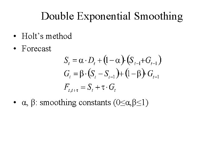
Double Exponential Smoothing • Holt’s method • Forecast • α, β: smoothing constants (0≤α, β≤ 1)

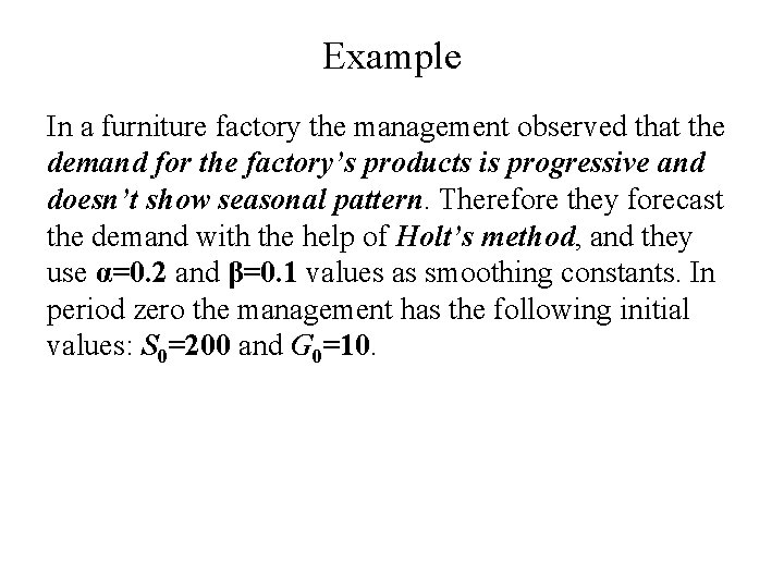
Example In a furniture factory the management observed that the demand for the factory’s products is progressive and doesn’t show seasonal pattern. Therefore they forecast the demand with the help of Holt’s method, and they use α=0. 2 and β=0. 1 values as smoothing constants. In period zero the management has the following initial values: S 0=200 and G 0=10.

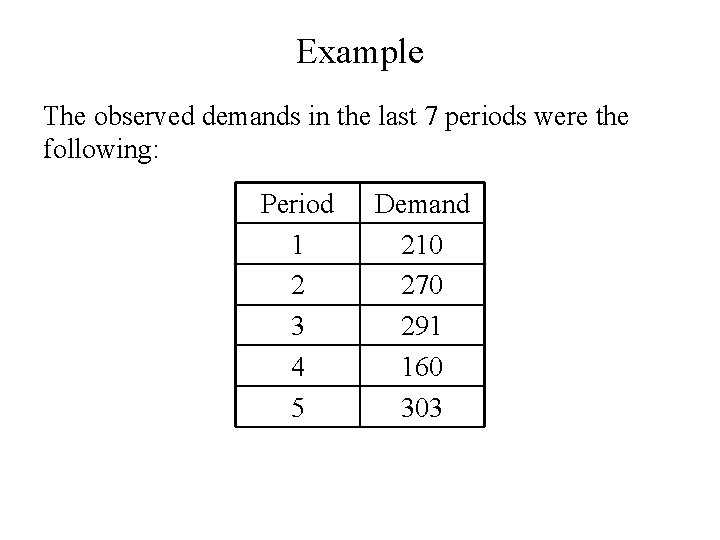
Example The observed demands in the last 7 periods were the following: Period 1 2 3 4 5 Demand 210 270 291 160 303

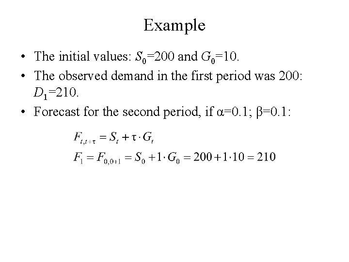
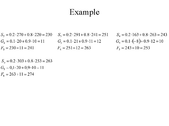
Example • The initial values: S 0=200 and G 0=10. • The observed demand in the first period was 200: D 1=210. • Forecast for the second period, if α=0. 1; β=0. 1:

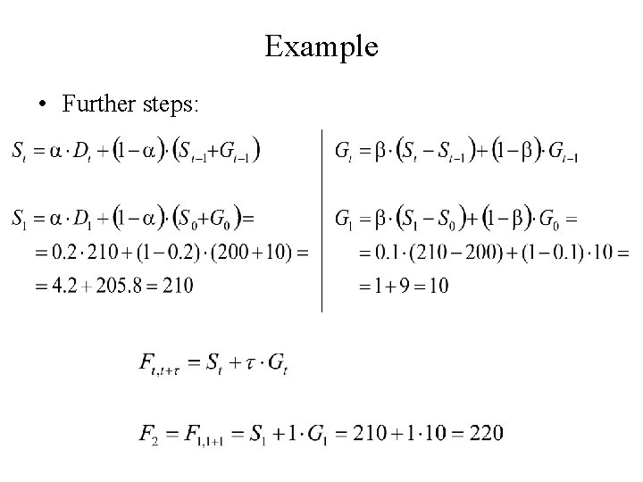
Example • Further steps:

Example

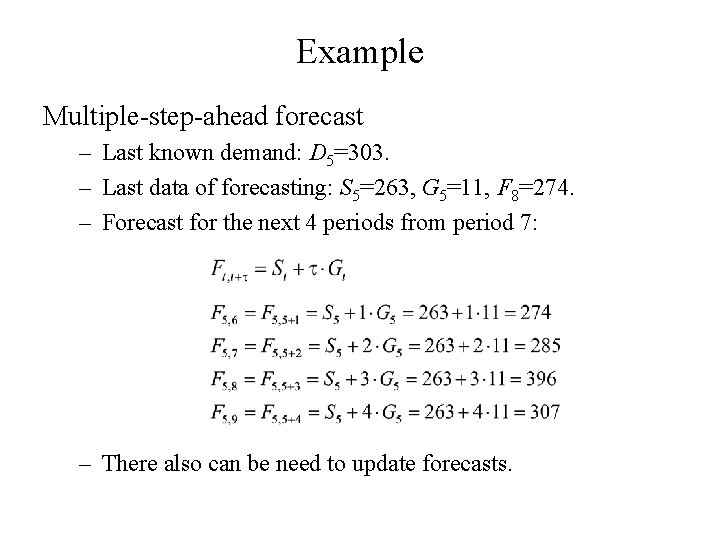
Example Multiple-step-ahead forecast – Last known demand: D 5=303. – Last data of forecasting: S 5=263, G 5=11, F 8=274. – Forecast for the next 4 periods from period 7: – There also can be need to update forecasts.

Evaluating Forecasts • There almost always errors in forecasts – Random effects, noises – Inappropriate forecasting methods • Analysis of – the size of forecasting errors – the validity of forecasting models

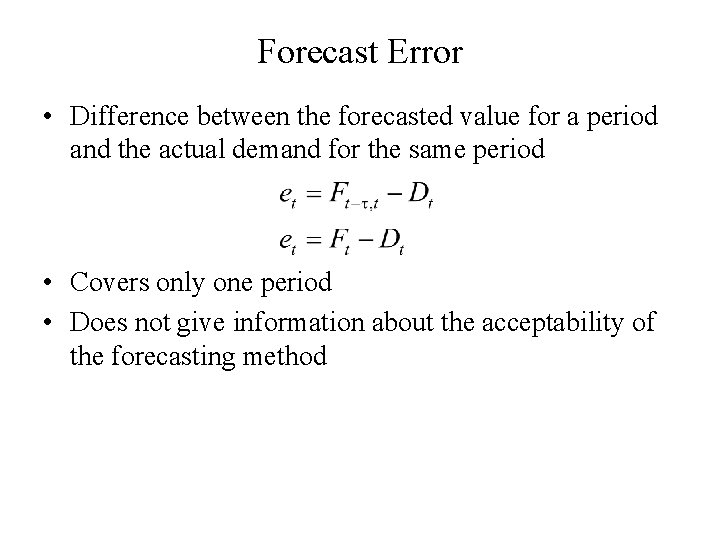
Forecast Error • Difference between the forecasted value for a period and the actual demand for the same period • Covers only one period • Does not give information about the acceptability of the forecasting method

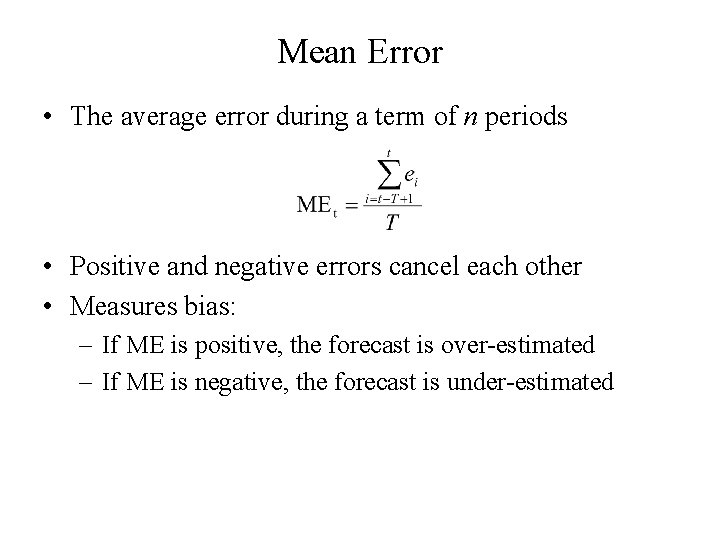
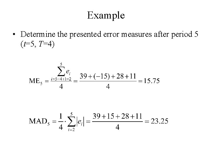
Mean Error • The average error during a term of n periods • Positive and negative errors cancel each other • Measures bias: – If ME is positive, the forecast is over-estimated – If ME is negative, the forecast is under-estimated

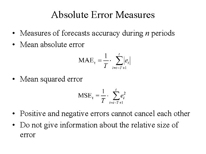
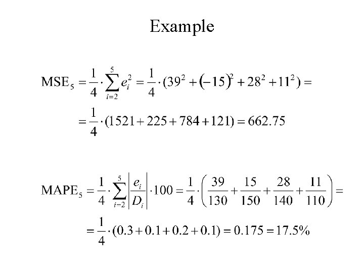
Absolute Error Measures • Measures of forecasts accuracy during n periods • Mean absolute error • Mean squared error • Positive and negative errors cannot cancel each other • Do not give information about the relative size of error

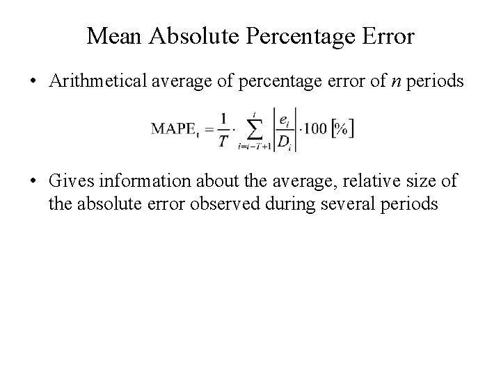
Mean Absolute Percentage Error • Arithmetical average of percentage error of n periods • Gives information about the average, relative size of the absolute error observed during several periods

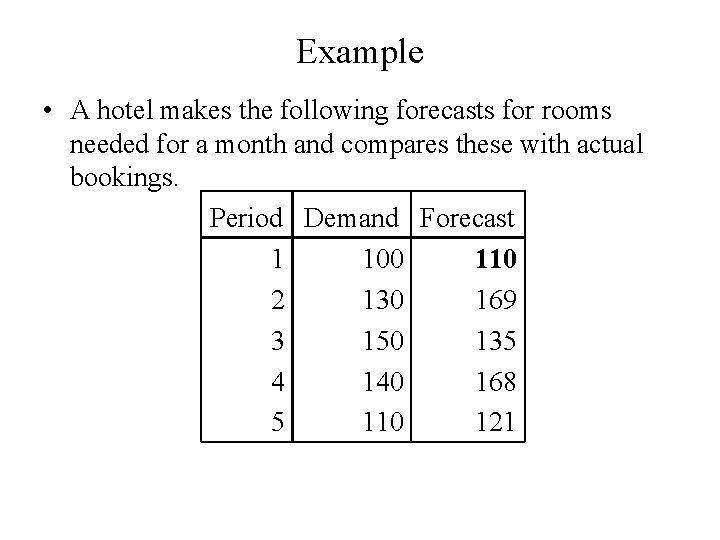
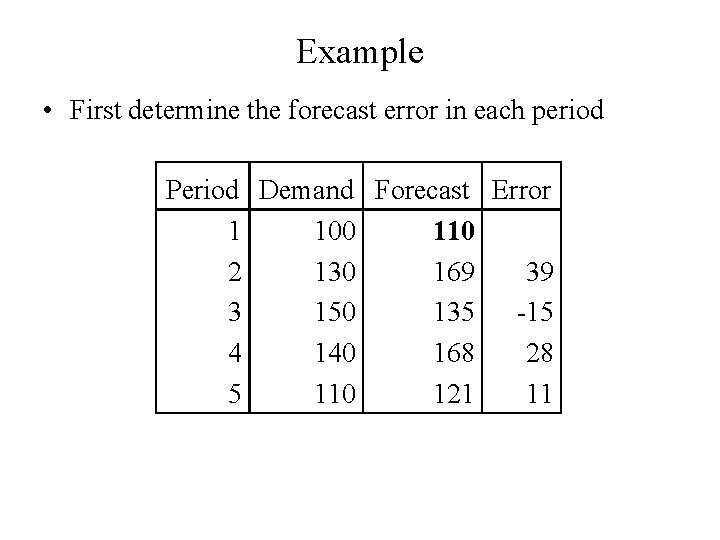
Example • A hotel makes the following forecasts for rooms needed for a month and compares these with actual bookings. Period Demand Forecast 1 100 110 2 130 169 3 150 135 4 140 168 5 110 121

Example • First determine the forecast error in each period Period Demand Forecast Error 1 100 110 2 130 169 39 3 150 135 -15 4 140 168 28 5 110 121 11

Example • Determine the presented error measures after period 5 (t=5, T=4)

Example

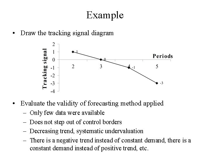
Validity of Forecasting Method • Analyzing the validity of the forecasting method used • Signs that forecast – is inappropriate – will be inappropriate in the immediate future • Tracking signal will be used • Monitoring – the size of tracking signal values – the tendency of tracking signal values

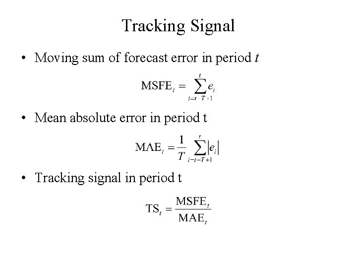
Tracking Signal • Moving sum of forecast error in period t • Mean absolute error in period t • Tracking signal in period t

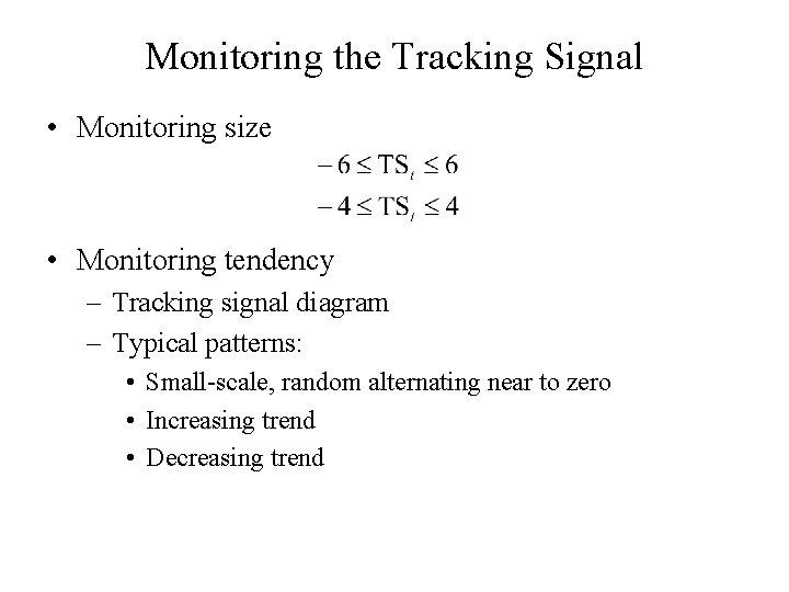
Monitoring the Tracking Signal • Monitoring size • Monitoring tendency – Tracking signal diagram – Typical patterns: • Small-scale, random alternating near to zero • Increasing trend • Decreasing trend

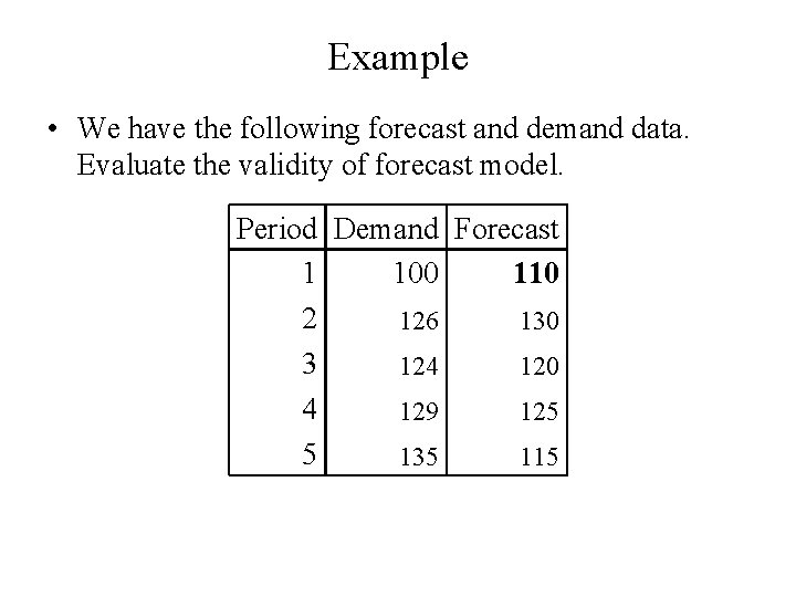
Example • We have the following forecast and demand data. Evaluate the validity of forecast model. Period Demand Forecast 1 100 110 2 126 130 3 124 120 4 129 125 5 135 115

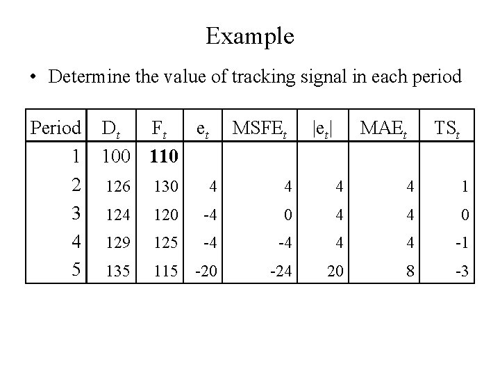
Example • Determine the value of tracking signal in each period Period 1 2 3 4 5 Dt Ft et 100 110 MSFEt |et| MAEt TSt 126 130 4 4 1 124 120 -4 0 4 4 0 129 125 -4 -4 4 4 -1 135 115 -20 -24 20 8 -3

Example • Draw the tracking signal diagram • Evaluate the validity of forecasting method applied – – Only few data were available Does not step out of control borders Decreasing trend, systematic undervaluation There is a negative trend instead of constant demand, there is a constant demand instead of positive trend, etc.