Operations Management Forecasting Chapter 4 Power Point presentation

Operations Management Forecasting Chapter 4 Power. Point presentation to accompany Heizer/Render – Principles of Operations Management, 5 e, and Operations Management, 7 e 1 © 2004 by Prentice Hall, Inc. , Upper Saddle River, N. J. 07458

Outline ¨ ¨ WHAT IS FORECASTING? TYPES OF FORECASTS THE STRATEGIC IMPORTANCE OF FORECASTING APPROACHES ¨ ¨ Overview of Qualitative Methods Overview of Quantitative Methods ¨ ¨ ¨ ¨ Naïve Approach Moving Averages Exponential Smoothing with Trend Adjustment Trend Projections Seasonal Variations in Data Cyclic Variations in Data ¨ TIME-SERIES FORECASTING ¨ ASSOCIATIVE FORECASTING METHODS: REGRESSION AND CORRELATION ANALYSIS ¨ MONITORING AND CONTROLLING FORECASTS Power. Point presentation to accompany Heizer/Render – Principles of Operations Management, 5 e, and Operations Management, 7 e 2 © 2004 by Prentice Hall, Inc. , Upper Saddle River, N. J. 07458

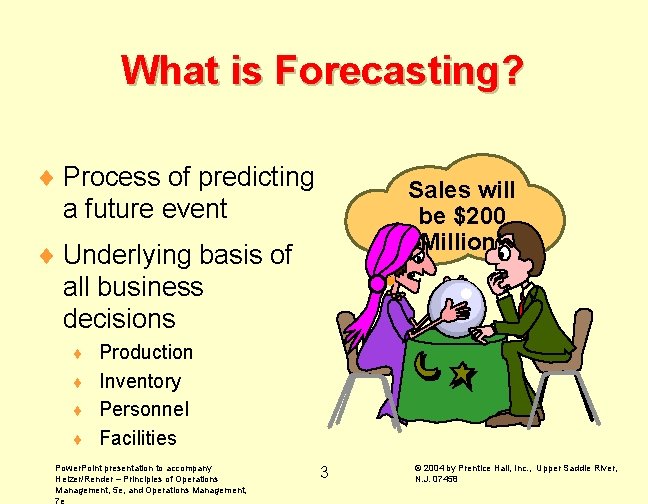
What is Forecasting? ¨ Process of predicting a future event Sales will be $200 Million! ¨ Underlying basis of all business decisions Production ¨ Inventory ¨ Personnel ¨ Facilities ¨ Power. Point presentation to accompany Heizer/Render – Principles of Operations Management, 5 e, and Operations Management, 7 e 3 © 2004 by Prentice Hall, Inc. , Upper Saddle River, N. J. 07458

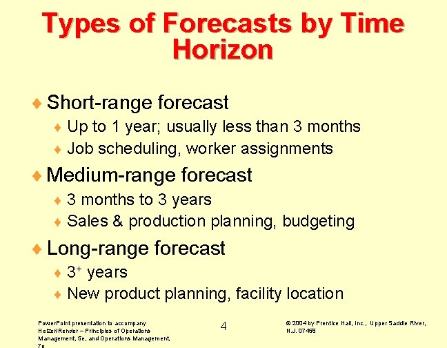
Types of Forecasts by Time Horizon ¨ Short-range forecast ¨ Up to 1 year; usually less than 3 months ¨ Job scheduling, worker assignments ¨ Medium-range forecast ¨ 3 months to 3 years ¨ Sales & production planning, budgeting ¨ Long-range forecast ¨ 3+ years ¨ New product planning, facility location Power. Point presentation to accompany Heizer/Render – Principles of Operations Management, 5 e, and Operations Management, 7 e 4 © 2004 by Prentice Hall, Inc. , Upper Saddle River, N. J. 07458

Short-term vs. Longer-term Forecasting ¨ Medium/long range forecasts deal with more comprehensive issues and support management decisions regarding planning and products, plants and processes. ¨ Short-term forecasting usually employs different methodologies than longerterm forecasting ¨ Short-term forecasts tend to be more accurate than longer-term forecasts. Power. Point presentation to accompany Heizer/Render – Principles of Operations Management, 5 e, and Operations Management, 7 e 5 © 2004 by Prentice Hall, Inc. , Upper Saddle River, N. J. 07458

Influence of Product Life Cycle Introduction, Growth, Maturity, Decline ¨ Stages of introduction and growth require longer forecasts than maturity and decline ¨ Forecasts useful in projecting staffing levels, ¨ inventory levels, and ¨ factory capacity ¨ as product passes through life cycle stages Power. Point presentation to accompany Heizer/Render – Principles of Operations Management, 5 e, and Operations Management, 7 e 6 © 2004 by Prentice Hall, Inc. , Upper Saddle River, N. J. 07458

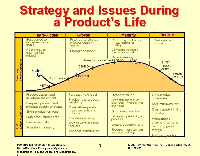
Strategy and Issues During a Product’s Life Company Strategy/Issues Introduction Maturity Growth Best period to increase market share Practical to change price or quality image R&D product engineering critical Strengthen niche Poor time to change image, price, or quality Competitive costs become critical Defend market Fax position Drive-thru restaurants machines CD-ROM Sales Cost control critical 3 1/2” Floppy disks Station wagons Internet Color copiers Decline HDTV OM Strategy/Issues Product design and development critical Frequent product and process design changes Forecasting critical Standardization Product and process reliability Less rapid product changes - more minor changes Short production runs Competitive product improvements and options High production costs Increase capacity Limited models Increasing stability of process Shift toward product focused Long production runs Enhance distribution Product improvement and cost cutting Attention to quality Power. Point presentation to accompany Heizer/Render – Principles of Operations Management, 5 e, and Operations Management, 7 e 7 Optimum capacity Little product differentiation Cost minimization Over capacity in the industry Prune line to eliminate items not returning good margin Reduce capacity © 2004 by Prentice Hall, Inc. , Upper Saddle River, N. J. 07458

Types of Forecasts ¨ Economic forecasts ¨ Address business cycle, e. g. , inflation rate, money supply etc. ¨ Technological forecasts ¨ Predict rate of technological progress ¨ Predict acceptance of new product ¨ Demand forecasts ¨ Predict sales of existing product Power. Point presentation to accompany Heizer/Render – Principles of Operations Management, 5 e, and Operations Management, 7 e 8 © 2004 by Prentice Hall, Inc. , Upper Saddle River, N. J. 07458

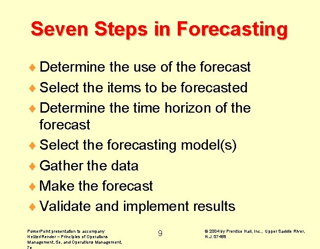
Seven Steps in Forecasting ¨ Determine the use of the forecast ¨ Select the items to be forecasted ¨ Determine the time horizon of the forecast ¨ Select the forecasting model(s) ¨ Gather the data ¨ Make the forecast ¨ Validate and implement results Power. Point presentation to accompany Heizer/Render – Principles of Operations Management, 5 e, and Operations Management, 7 e 9 © 2004 by Prentice Hall, Inc. , Upper Saddle River, N. J. 07458

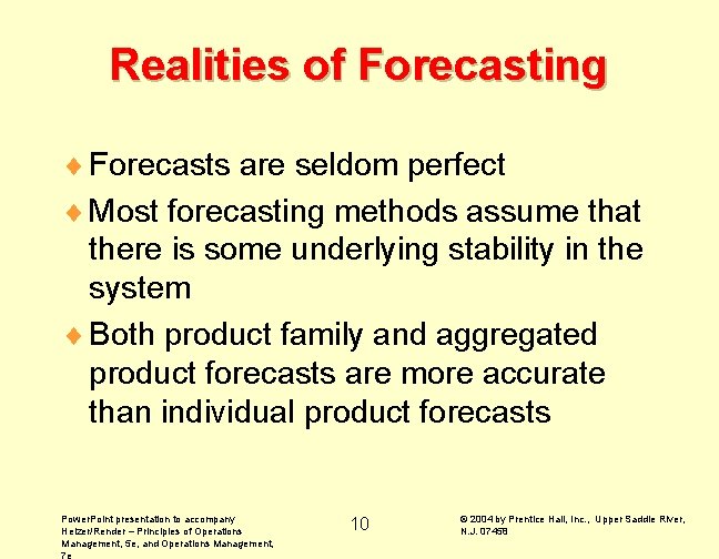
Realities of Forecasting ¨ Forecasts are seldom perfect ¨ Most forecasting methods assume that there is some underlying stability in the system ¨ Both product family and aggregated product forecasts are more accurate than individual product forecasts Power. Point presentation to accompany Heizer/Render – Principles of Operations Management, 5 e, and Operations Management, 7 e 10 © 2004 by Prentice Hall, Inc. , Upper Saddle River, N. J. 07458

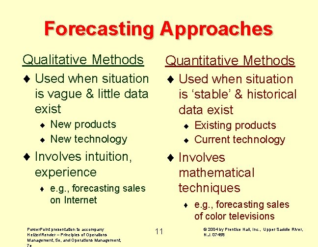
Forecasting Approaches Qualitative Methods Quantitative Methods ¨ Used when situation is vague & little data exist ¨ Used when situation is ‘stable’ & historical data exist New products ¨ New technology Existing products ¨ Current technology ¨ ¨ ¨ Involves intuition, experience ¨ ¨ Involves mathematical techniques e. g. , forecasting sales on Internet Power. Point presentation to accompany Heizer/Render – Principles of Operations Management, 5 e, and Operations Management, 7 e ¨ 11 e. g. , forecasting sales of color televisions © 2004 by Prentice Hall, Inc. , Upper Saddle River, N. J. 07458

Overview of Qualitative Methods ¨ Jury of executive opinion ¨ Pool opinions of high-level executives, sometimes augment by statistical models ¨ Delphi method ¨ Panel of experts, queried iteratively ¨ Sales force composite ¨ Estimates from individual salespersons are reviewed for reasonableness, then aggregated ¨ Consumer Market Survey Power. Point presentation to accompany Heizer/Render – Principles of Operations Management, 5 e, and Operations Management, 7 e ¨ Ask the customer 12 © 2004 by Prentice Hall, Inc. , Upper Saddle River, N. J. 07458

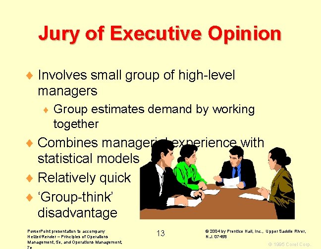
Jury of Executive Opinion ¨ Involves small group of high-level managers ¨ Group estimates demand by working together ¨ Combines managerial experience with statistical models ¨ Relatively quick ¨ ‘Group-think’ disadvantage Power. Point presentation to accompany Heizer/Render – Principles of Operations Management, 5 e, and Operations Management, 7 e 13 © 2004 by Prentice Hall, Inc. , Upper Saddle River, N. J. 07458 © 1995 Corel Corp.

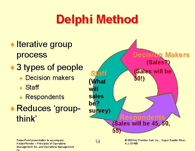
Delphi Method ¨ Iterative group process ¨ 3 types of people Decision makers ¨ Staff ¨ Respondents ¨ ¨ Reduces ‘groupthink’ Power. Point presentation to accompany Heizer/Render – Principles of Operations Management, 5 e, and Operations Management, 7 e Decision Makers Staff (What will sales be? survey) (Sales? ) (Sales will be 50!) Respondents (Sales will be 45, 50, 55) 14 © 2004 by Prentice Hall, Inc. , Upper Saddle River, N. J. 07458

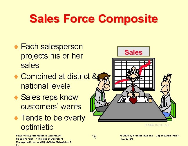
Sales Force Composite ¨ Each salesperson projects his or her sales ¨ Combined at district & national levels ¨ Sales reps know customers’ wants ¨ Tends to be overly optimistic Power. Point presentation to accompany Heizer/Render – Principles of Operations Management, 5 e, and Operations Management, 7 e 15 Sales © 1995 Corel Corp. © 2004 by Prentice Hall, Inc. , Upper Saddle River, N. J. 07458

Consumer Market Survey ¨ Ask customers about purchasing plans ¨ What consumers say, and what they actually do are often different ¨ Sometimes difficult to answer Power. Point presentation to accompany Heizer/Render – Principles of Operations Management, 5 e, and Operations Management, 7 e How many hours will you use the Internet next week? © 1995 Corel Corp. 16 © 2004 by Prentice Hall, Inc. , Upper Saddle River, N. J. 07458

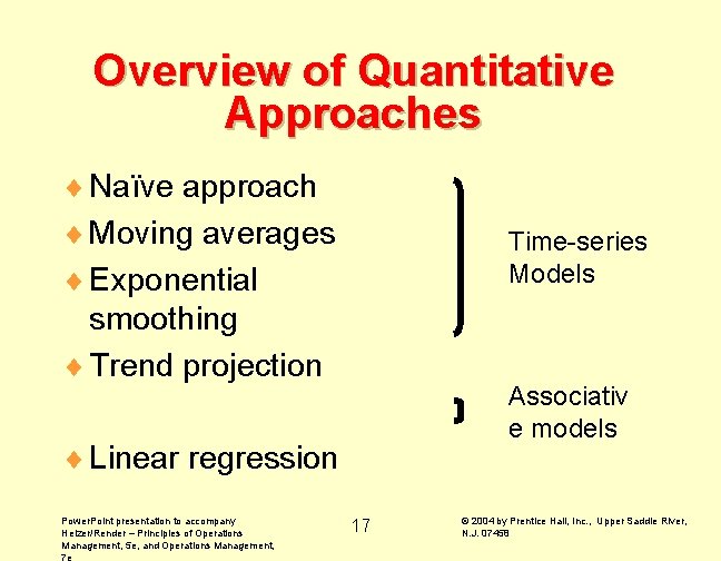
Overview of Quantitative Approaches ¨ Naïve approach ¨ Moving averages ¨ Exponential smoothing ¨ Trend projection Time-series Models Associativ e models ¨ Linear regression Power. Point presentation to accompany Heizer/Render – Principles of Operations Management, 5 e, and Operations Management, 7 e 17 © 2004 by Prentice Hall, Inc. , Upper Saddle River, N. J. 07458

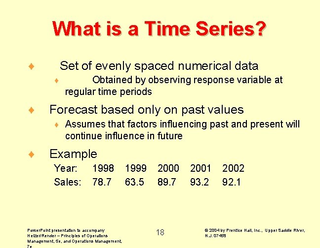
What is a Time Series? ¨ Set of evenly spaced numerical data ¨ ¨ Forecast based only on past values ¨ ¨ Obtained by observing response variable at regular time periods Assumes that factors influencing past and present will continue influence in future Example Year: Sales: 1998 78. 7 Power. Point presentation to accompany Heizer/Render – Principles of Operations Management, 5 e, and Operations Management, 7 e 1999 63. 5 2000 89. 7 18 2001 93. 2 2002 92. 1 © 2004 by Prentice Hall, Inc. , Upper Saddle River, N. J. 07458

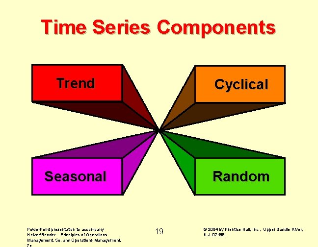
Time Series Components Trend Cyclical Seasonal Random Power. Point presentation to accompany Heizer/Render – Principles of Operations Management, 5 e, and Operations Management, 7 e 19 © 2004 by Prentice Hall, Inc. , Upper Saddle River, N. J. 07458

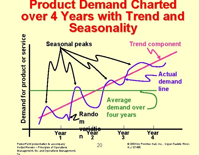
Demand for product or service Product Demand Charted over 4 Years with Trend and Seasonality Seasonal peaks Trend component Actual demand line Year 1 Power. Point presentation to accompany Heizer/Render – Principles of Operations Management, 5 e, and Operations Management, 7 e Rando m variatio Year n 2 20 Average demand over four years Year 3 Year 4 © 2004 by Prentice Hall, Inc. , Upper Saddle River, N. J. 07458

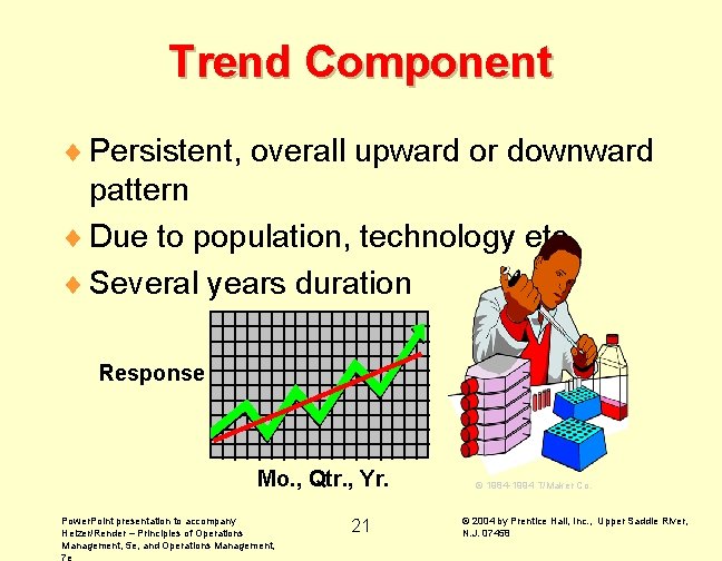
Trend Component ¨ Persistent, overall upward or downward pattern ¨ Due to population, technology etc. ¨ Several years duration Response Mo. , Qtr. , Yr. Power. Point presentation to accompany Heizer/Render – Principles of Operations Management, 5 e, and Operations Management, 7 e 21 © 1984 -1994 T/Maker Co. © 2004 by Prentice Hall, Inc. , Upper Saddle River, N. J. 07458

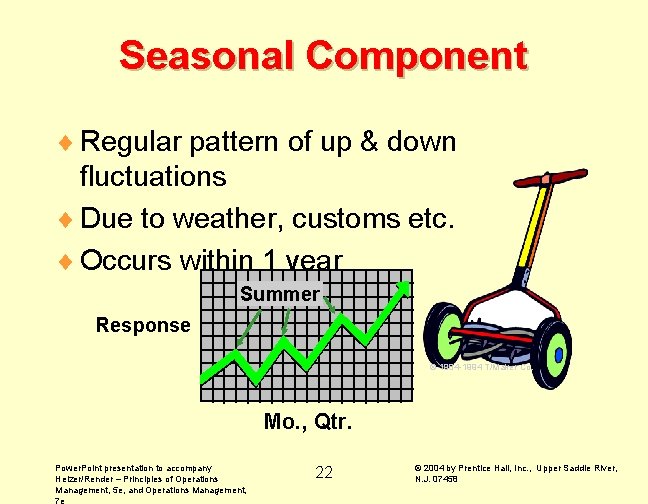
Seasonal Component ¨ Regular pattern of up & down fluctuations ¨ Due to weather, customs etc. ¨ Occurs within 1 year Summer Response © 1984 -1994 T/Maker Co. Mo. , Qtr. Power. Point presentation to accompany Heizer/Render – Principles of Operations Management, 5 e, and Operations Management, 7 e 22 © 2004 by Prentice Hall, Inc. , Upper Saddle River, N. J. 07458

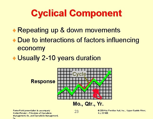
Cyclical Component ¨ Repeating up & down movements ¨ Due to interactions of factors influencing economy ¨ Usually 2 -10 years duration Cycle Response Mo. , Qtr. , Yr. Power. Point presentation to accompany Heizer/Render – Principles of Operations Management, 5 e, and Operations Management, 7 e 23 © 2004 by Prentice Hall, Inc. , Upper Saddle River, N. J. 07458

Random Component ¨ Erratic, unsystematic, ‘residual’ fluctuations © 1984 -1994 T/Maker Co. ¨ Due to random variation or unforeseen events ¨ Union strike ¨ Tornado ¨ Short duration & nonrepeating Power. Point presentation to accompany Heizer/Render – Principles of Operations Management, 5 e, and Operations Management, 7 e 24 © 2004 by Prentice Hall, Inc. , Upper Saddle River, N. J. 07458

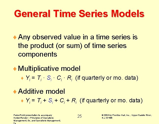
General Time Series Models ¨ Any observed value in a time series is the product (or sum) of time series components ¨ Multiplicative model ¨ Yi = Ti · Si · Ci · Ri (if quarterly or mo. data) ¨ Additive model ¨ Yi = Ti + Si + Ci + Ri (if quarterly or mo. data) Power. Point presentation to accompany Heizer/Render – Principles of Operations Management, 5 e, and Operations Management, 7 e 25 © 2004 by Prentice Hall, Inc. , Upper Saddle River, N. J. 07458

Naive Approach ¨ Assumes demand in next period is the same as demand in most recent period ¨ e. g. , If May sales were 48, then June sales will be 48 ¨ Sometimes cost effective & efficient © 1995 Corel Corp. Power. Point presentation to accompany Heizer/Render – Principles of Operations Management, 5 e, and Operations Management, 7 e 26 © 2004 by Prentice Hall, Inc. , Upper Saddle River, N. J. 07458

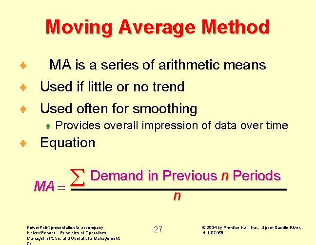
Moving Average Method ¨ MA is a series of arithmetic means ¨ Used if little or no trend ¨ Used often for smoothing ¨ Provides overall impression of data over time ¨ Equation Demand in Previous n Periods MA n Power. Point presentation to accompany Heizer/Render – Principles of Operations Management, 5 e, and Operations Management, 7 e 27 © 2004 by Prentice Hall, Inc. , Upper Saddle River, N. J. 07458

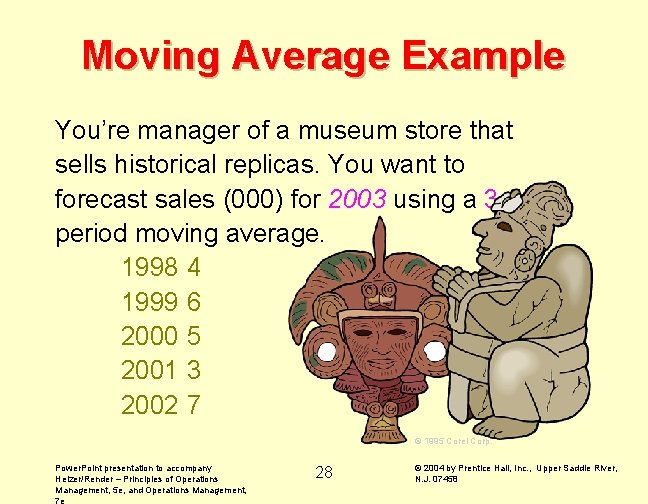
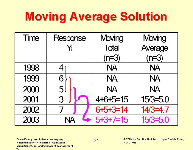
Moving Average Example You’re manager of a museum store that sells historical replicas. You want to forecast sales (000) for 2003 using a 3 period moving average. 1998 4 1999 6 2000 5 2001 3 2002 7 © 1995 Corel Corp. Power. Point presentation to accompany Heizer/Render – Principles of Operations Management, 5 e, and Operations Management, 7 e 28 © 2004 by Prentice Hall, Inc. , Upper Saddle River, N. J. 07458

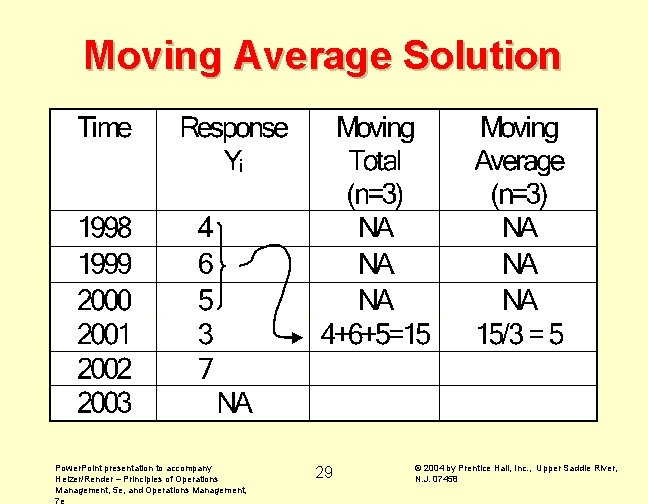
Moving Average Solution Power. Point presentation to accompany Heizer/Render – Principles of Operations Management, 5 e, and Operations Management, 7 e 29 © 2004 by Prentice Hall, Inc. , Upper Saddle River, N. J. 07458

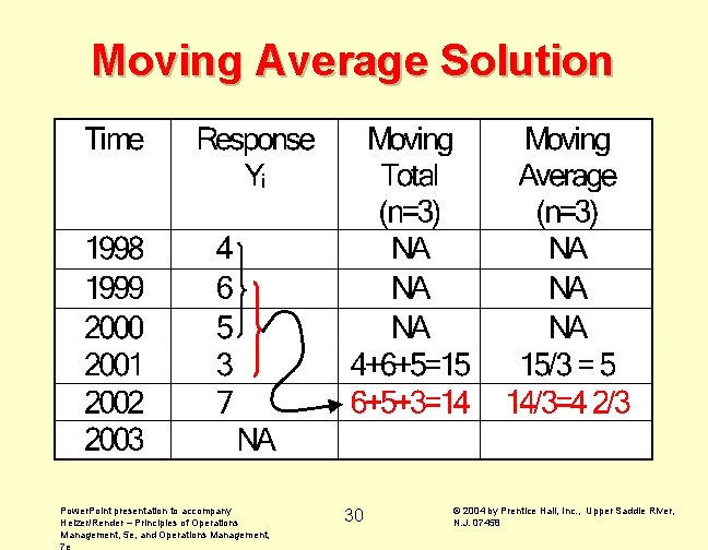
Moving Average Solution Power. Point presentation to accompany Heizer/Render – Principles of Operations Management, 5 e, and Operations Management, 7 e 30 © 2004 by Prentice Hall, Inc. , Upper Saddle River, N. J. 07458

Moving Average Solution Power. Point presentation to accompany Heizer/Render – Principles of Operations Management, 5 e, and Operations Management, 7 e 31 © 2004 by Prentice Hall, Inc. , Upper Saddle River, N. J. 07458

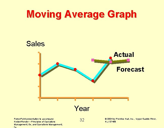
Moving Average Graph Sales 8 Actual 6 Forecast 4 2 95 96 Power. Point presentation to accompany Heizer/Render – Principles of Operations Management, 5 e, and Operations Management, 7 e 97 98 Year 32 99 00 © 2004 by Prentice Hall, Inc. , Upper Saddle River, N. J. 07458

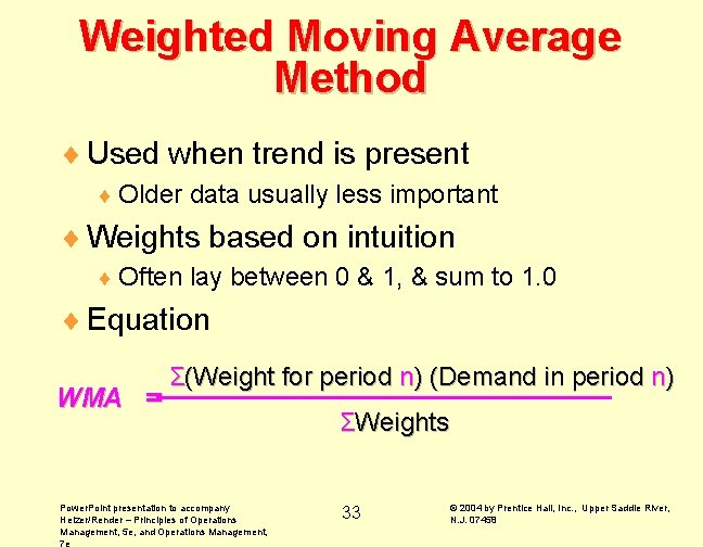
Weighted Moving Average Method ¨ Used when trend is present ¨ Older data usually less important ¨ Weights based on intuition ¨ Often lay between 0 & 1, & sum to 1. 0 ¨ Equation WMA = Σ(Weight for period n) (Demand in period n) Power. Point presentation to accompany Heizer/Render – Principles of Operations Management, 5 e, and Operations Management, 7 e ΣWeights 33 © 2004 by Prentice Hall, Inc. , Upper Saddle River, N. J. 07458

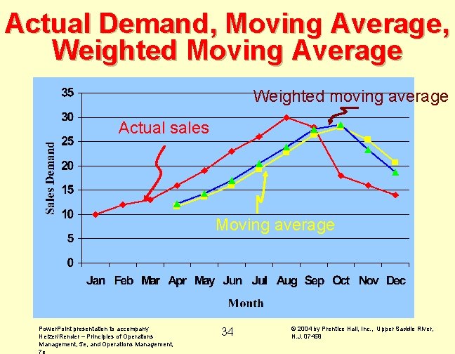
Actual Demand, Moving Average, Weighted Moving Average Weighted moving average Actual sales Moving average Power. Point presentation to accompany Heizer/Render – Principles of Operations Management, 5 e, and Operations Management, 7 e 34 © 2004 by Prentice Hall, Inc. , Upper Saddle River, N. J. 07458

Disadvantages of Moving Average Methods ¨ Increasing n makes forecast less sensitive to changes ¨ Do not forecast trend well ¨ Require much historical data © 1984 -1994 T/Maker Co. Power. Point presentation to accompany Heizer/Render – Principles of Operations Management, 5 e, and Operations Management, 7 e 35 © 2004 by Prentice Hall, Inc. , Upper Saddle River, N. J. 07458

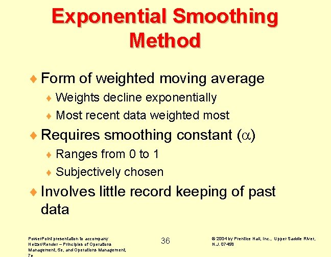
Exponential Smoothing Method ¨ Form of weighted moving average ¨ Weights decline exponentially ¨ Most recent data weighted most ¨ Requires smoothing constant ( ) ¨ Ranges from 0 to 1 ¨ Subjectively chosen ¨ Involves little record keeping of past data Power. Point presentation to accompany Heizer/Render – Principles of Operations Management, 5 e, and Operations Management, 7 e 36 © 2004 by Prentice Hall, Inc. , Upper Saddle River, N. J. 07458

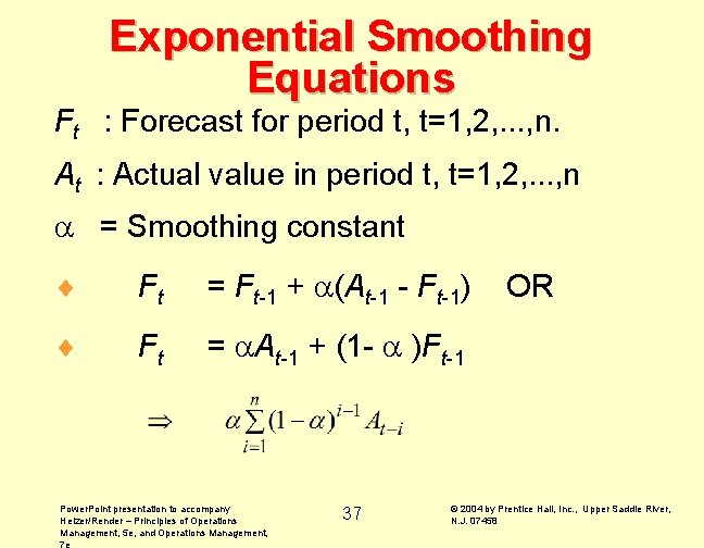
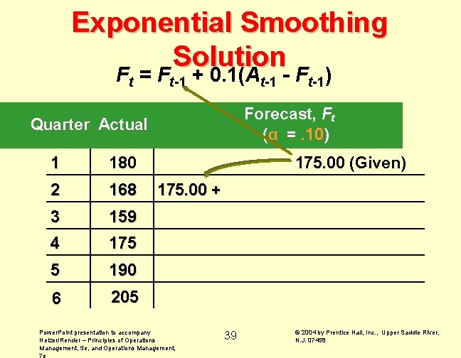
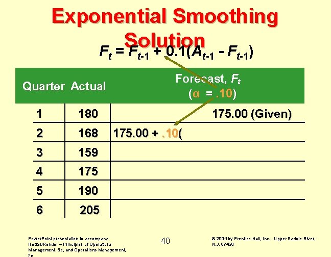
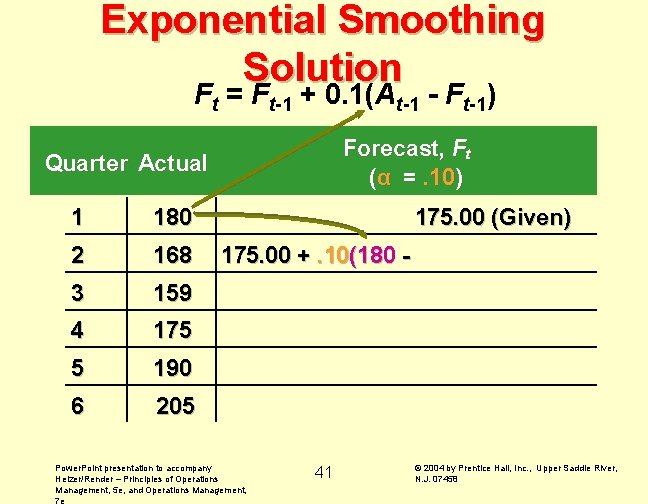
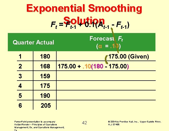
Exponential Smoothing Equations Ft : Forecast for period t, t=1, 2, . . . , n. At : Actual value in period t, t=1, 2, . . . , n = Smoothing constant ¨ Ft = Ft-1 + (At-1 - Ft-1) ¨ Ft = At-1 + (1 - )Ft-1 Power. Point presentation to accompany Heizer/Render – Principles of Operations Management, 5 e, and Operations Management, 7 e 37 OR © 2004 by Prentice Hall, Inc. , Upper Saddle River, N. J. 07458

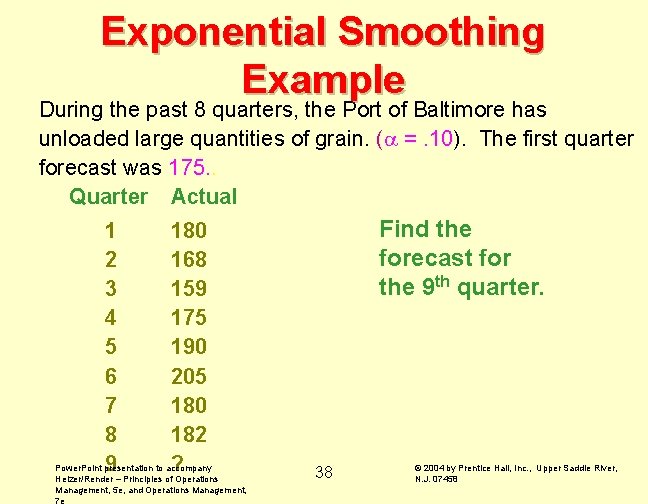
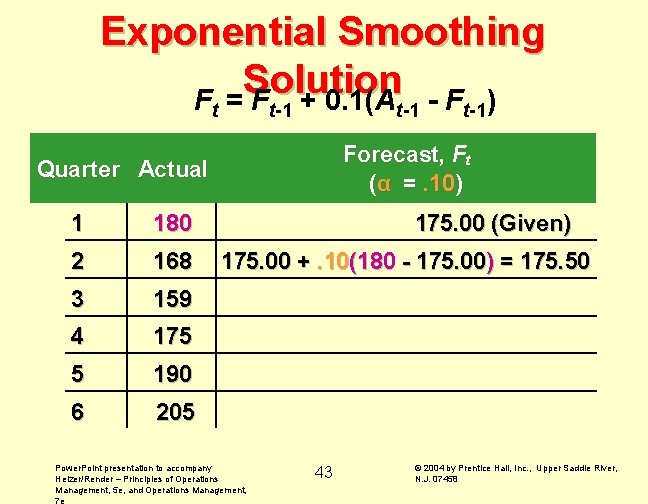
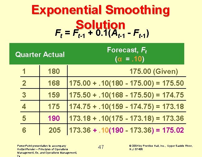
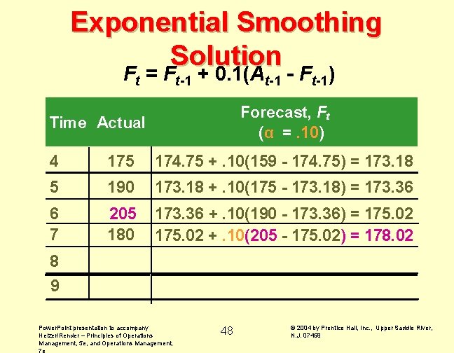
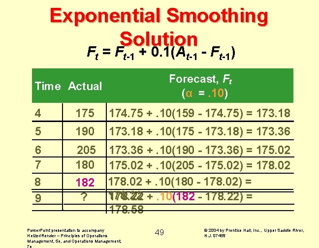
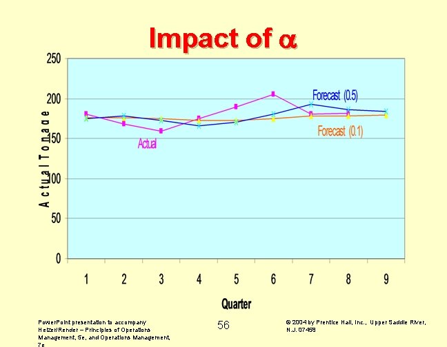
Exponential Smoothing Example During the past 8 quarters, the Port of Baltimore has unloaded large quantities of grain. ( =. 10). The first quarter forecast was 175. . Quarter Actual 1 180 2 168 3 159 4 175 5 190 6 205 7 180 8 182 Power. Point presentation to accompany 9 ? Heizer/Render – Principles of Operations Management, 5 e, and Operations Management, 7 e Find the forecast for the 9 th quarter. 38 © 2004 by Prentice Hall, Inc. , Upper Saddle River, N. J. 07458

Exponential Smoothing Solution Ft = Ft-1 + 0. 1(At-1 - Ft-1) Forecast, Ft (α =. 10) Quarter Actual 1 180 2 168 3 159 4 175 5 190 6 205 175. 00 (Given) 175. 00 + Power. Point presentation to accompany Heizer/Render – Principles of Operations Management, 5 e, and Operations Management, 7 e 39 © 2004 by Prentice Hall, Inc. , Upper Saddle River, N. J. 07458

Exponential Smoothing Solution F = F + 0. 1(A - F ) t t-1 Forecast, Ft (α =. 10) Quarter Actual Actua 1 180 2 168 3 159 4 175 5 190 6 205 t-1 175. 00 (Given) 175. 00 +. 10( Power. Point presentation to accompany Heizer/Render – Principles of Operations Management, 5 e, and Operations Management, 7 e 40 © 2004 by Prentice Hall, Inc. , Upper Saddle River, N. J. 07458

Exponential Smoothing Solution Ft = Ft-1 + 0. 1(At-1 - Ft-1) Forecast, Ft (α =. 10) Quarter Actual 1 180 2 168 3 159 4 175 5 190 6 205 175. 00 (Given) 175. 00 +. 10(180 - Power. Point presentation to accompany Heizer/Render – Principles of Operations Management, 5 e, and Operations Management, 7 e 41 © 2004 by Prentice Hall, Inc. , Upper Saddle River, N. J. 07458

Exponential Smoothing Ft =Solution Ft-1 + 0. 1(At-1 - Ft-1) Forecast, Ft (α =. 10) Quarter Actual 1 180 2 168 3 159 4 175 5 190 6 205 175. 00 (Given) 175. 00 +. 10(180 - 175. 00) Power. Point presentation to accompany Heizer/Render – Principles of Operations Management, 5 e, and Operations Management, 7 e 42 © 2004 by Prentice Hall, Inc. , Upper Saddle River, N. J. 07458

Exponential Smoothing Solution F = F + 0. 1(A - F ) t t-1 Forecast, Ft (α =. 10) Quarter Actual 1 180 2 168 3 159 4 175 5 190 6 205 t-1 175. 00 (Given) 175. 00 +. 10(180 - 175. 00) = 175. 50 Power. Point presentation to accompany Heizer/Render – Principles of Operations Management, 5 e, and Operations Management, 7 e 43 © 2004 by Prentice Hall, Inc. , Upper Saddle River, N. J. 07458

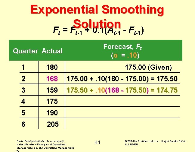
Exponential Smoothing Solution F = F + 0. 1(A - F ) t t-1 t-1 Forecast, Ft (α =. 10) Quarter Actual 1 180 175. 00 (Given) 2 168 175. 00 +. 10(180 - 175. 00) = 175. 50 3 159 175. 50 +. 10(168 - 175. 50) = 174. 75 4 175 5 190 6 205 Power. Point presentation to accompany Heizer/Render – Principles of Operations Management, 5 e, and Operations Management, 7 e 44 © 2004 by Prentice Hall, Inc. , Upper Saddle River, N. J. 07458

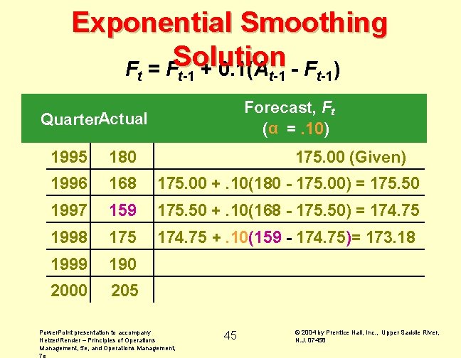
Exponential Smoothing Ft = FSolution t-1 + 0. 1(At-1 - Ft-1) Forecast, Ft (α =. 10) Quarter. Actual 1995 180 175. 00 (Given) 1996 168 175. 00 +. 10(180 - 175. 00) = 175. 50 1997 159 175. 50 +. 10(168 - 175. 50) = 174. 75 1998 175 174. 75 +. 10(159 - 174. 75)= 173. 18 1999 190 2000 205 Power. Point presentation to accompany Heizer/Render – Principles of Operations Management, 5 e, and Operations Management, 7 e 45 © 2004 by Prentice Hall, Inc. , Upper Saddle River, N. J. 07458

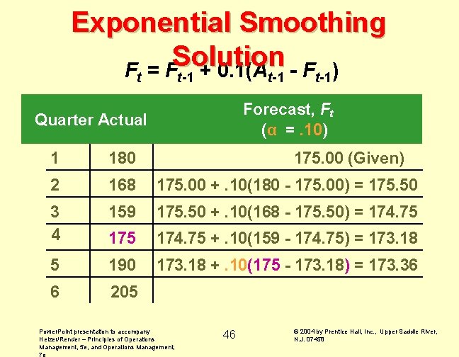
Exponential Smoothing Solution F = F + 0. 1(A - F ) t t-1 t-1 Forecast, Ft (α =. 10) Quarter Actual 1 180 175. 00 (Given) 2 168 175. 00 +. 10(180 - 175. 00) = 175. 50 3 4 159 175. 50 +. 10(168 - 175. 50) = 174. 75 +. 10(159 - 174. 75) = 173. 18 5 190 173. 18 +. 10(175 - 173. 18) = 173. 36 6 205 Power. Point presentation to accompany Heizer/Render – Principles of Operations Management, 5 e, and Operations Management, 7 e 46 © 2004 by Prentice Hall, Inc. , Upper Saddle River, N. J. 07458

Exponential Smoothing Solution Ft = Ft-1 + 0. 1(At-1 - Ft-1) Forecast, Ft (α =. 10) Quarter Actual 1 180 175. 00 (Given) 2 168 175. 00 +. 10(180 - 175. 00) = 175. 50 3 159 175. 50 +. 10(168 - 175. 50) = 174. 75 4 175 174. 75 +. 10(159 - 174. 75) = 173. 18 5 190 173. 18 +. 10(175 - 173. 18) = 173. 36 6 205 173. 36 +. 10(190 - 173. 36) = 175. 02 Power. Point presentation to accompany Heizer/Render – Principles of Operations Management, 5 e, and Operations Management, 7 e 47 © 2004 by Prentice Hall, Inc. , Upper Saddle River, N. J. 07458

Exponential Smoothing Solution Ft = Ft-1 + 0. 1(At-1 - Ft-1) Forecast, Ft (α =. 10) Time Actual 4 175 174. 75 +. 10(159 - 174. 75) = 173. 18 5 190 173. 18 +. 10(175 - 173. 18) = 173. 36 6 7 205 180 173. 36 +. 10(190 - 173. 36) = 175. 02 +. 10(205 - 175. 02) = 178. 02 8 9 Power. Point presentation to accompany Heizer/Render – Principles of Operations Management, 5 e, and Operations Management, 7 e 48 © 2004 by Prentice Hall, Inc. , Upper Saddle River, N. J. 07458

Exponential Smoothing Solution Ft = Ft-1 + 0. 1(At-1 - Ft-1) Forecast, Ft (α =. 10) Time Actual 4 175 174. 75 +. 10(159 - 174. 75) = 173. 18 5 190 173. 18 +. 10(175 - 173. 18) = 173. 36 6 7 205 180 8 9 182 ? 173. 36 +. 10(190 - 173. 36) = 175. 02 +. 10(205 - 175. 02) = 178. 02 +. 10(180 - 178. 02) = 178. 22 +. 10(182 - 178. 22) = 178. 58 Power. Point presentation to accompany Heizer/Render – Principles of Operations Management, 5 e, and Operations Management, 7 e 49 © 2004 by Prentice Hall, Inc. , Upper Saddle River, N. J. 07458

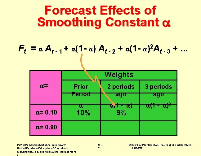
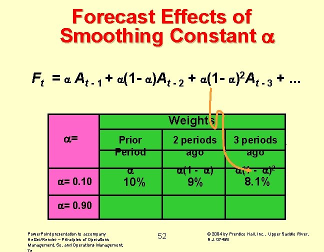
Forecast Effects of Smoothing Constant Ft = At - 1 + (1 - )At - 2 + (1 - )2 At - 3 +. . . Weights = = 0. 10 Prior Period 2 periods ago 3 periods ago (1 - )2 10% = 0. 90 Power. Point presentation to accompany Heizer/Render – Principles of Operations Management, 5 e, and Operations Management, 7 e 50 © 2004 by Prentice Hall, Inc. , Upper Saddle River, N. J. 07458

Forecast Effects of Smoothing Constant Ft = At - 1 + (1 - ) At - 2 + (1 - )2 At - 3 +. . . Weights = = 0. 10 Prior Period 2 periods ago 3 periods ago (1 - )2 9% 10% = 0. 90 Power. Point presentation to accompany Heizer/Render – Principles of Operations Management, 5 e, and Operations Management, 7 e 51 © 2004 by Prentice Hall, Inc. , Upper Saddle River, N. J. 07458

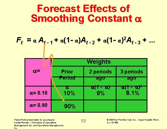
Forecast Effects of Smoothing Constant Ft = At - 1 + (1 - )At - 2 + (1 - )2 At - 3 +. . . Weights = = 0. 10 Prior Period 2 periods ago 3 periods ago (1 - )2 9% 10% 8. 1% = 0. 90 Power. Point presentation to accompany Heizer/Render – Principles of Operations Management, 5 e, and Operations Management, 7 e 52 © 2004 by Prentice Hall, Inc. , Upper Saddle River, N. J. 07458

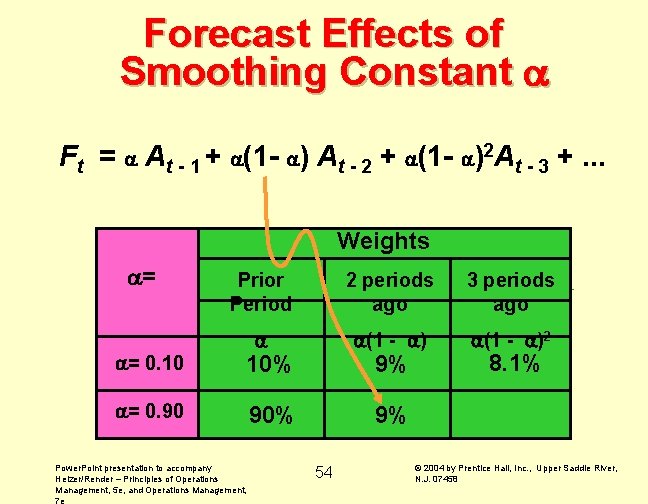
Forecast Effects of Smoothing Constant Ft = At - 1 + (1 - )At - 2 + (1 - )2 At - 3 +. . . Weights = Prior Period 2 periods ago 3 periods ago (1 - )2 = 0. 10 10% = 0. 90 90% Power. Point presentation to accompany Heizer/Render – Principles of Operations Management, 5 e, and Operations Management, 7 e 9% 53 8. 1% © 2004 by Prentice Hall, Inc. , Upper Saddle River, N. J. 07458

Forecast Effects of Smoothing Constant Ft = At - 1 + (1 - ) At - 2 + (1 - )2 At - 3 +. . . Weights = Prior Period 2 periods ago 3 periods ago (1 - )2 = 0. 10 10% = 0. 90 90% Power. Point presentation to accompany Heizer/Render – Principles of Operations Management, 5 e, and Operations Management, 7 e 9% 8. 1% 9% 54 © 2004 by Prentice Hall, Inc. , Upper Saddle River, N. J. 07458

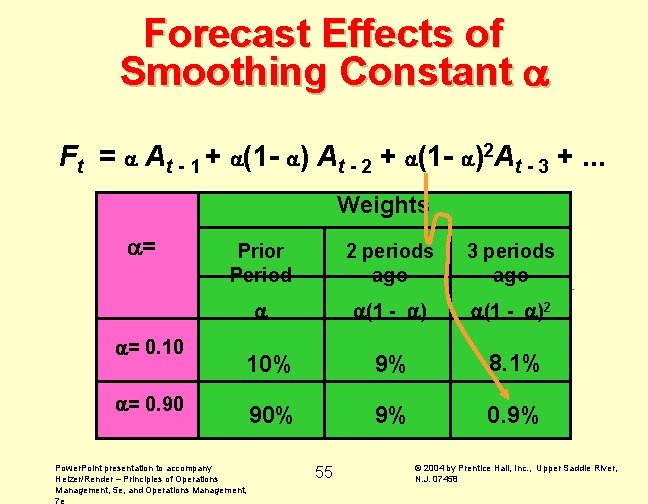
Forecast Effects of Smoothing Constant Ft = At - 1 + (1 - ) At - 2 + (1 - )2 At - 3 +. . . Weights = = 0. 10 Prior Period 2 periods ago 3 periods ago (1 - )2 10% 9% 8. 1% 90% 9% 0. 9% = 0. 90 Power. Point presentation to accompany Heizer/Render – Principles of Operations Management, 5 e, and Operations Management, 7 e 55 © 2004 by Prentice Hall, Inc. , Upper Saddle River, N. J. 07458

Impact of Power. Point presentation to accompany Heizer/Render – Principles of Operations Management, 5 e, and Operations Management, 7 e 56 © 2004 by Prentice Hall, Inc. , Upper Saddle River, N. J. 07458

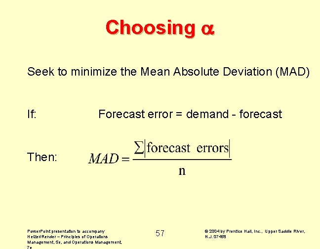
Choosing Seek to minimize the Mean Absolute Deviation (MAD) If: Forecast error = demand - forecast Then: Power. Point presentation to accompany Heizer/Render – Principles of Operations Management, 5 e, and Operations Management, 7 e 57 © 2004 by Prentice Hall, Inc. , Upper Saddle River, N. J. 07458

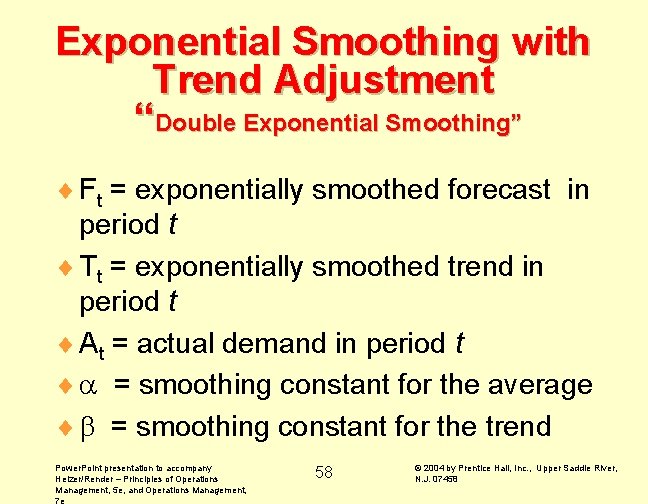
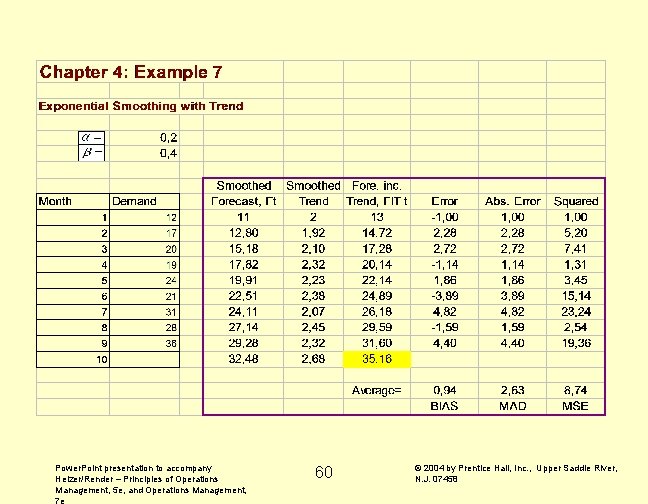
Exponential Smoothing with Trend Adjustment “Double Exponential Smoothing” ¨ Ft = exponentially smoothed forecast in period t ¨ Tt = exponentially smoothed trend in period t ¨ At = actual demand in period t ¨ = smoothing constant for the average ¨ = smoothing constant for the trend Power. Point presentation to accompany Heizer/Render – Principles of Operations Management, 5 e, and Operations Management, 7 e 58 © 2004 by Prentice Hall, Inc. , Upper Saddle River, N. J. 07458

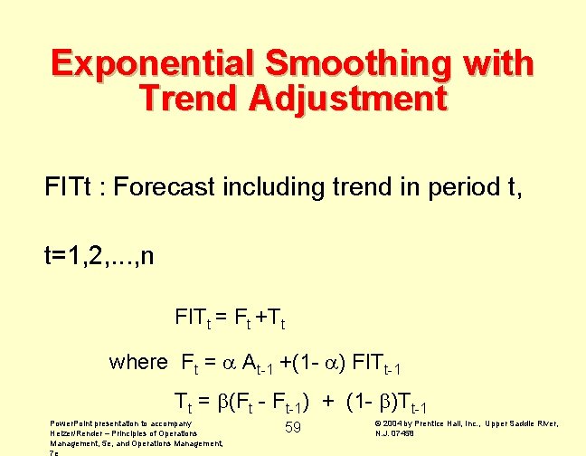
Exponential Smoothing with Trend Adjustment FITt : Forecast including trend in period t, t=1, 2, . . . , n FITt = Ft +Tt where Ft = At-1 +(1 - ) FITt-1 Tt = (Ft - Ft-1) + (1 - )Tt-1 Power. Point presentation to accompany Heizer/Render – Principles of Operations Management, 5 e, and Operations Management, 7 e 59 © 2004 by Prentice Hall, Inc. , Upper Saddle River, N. J. 07458

Power. Point presentation to accompany Heizer/Render – Principles of Operations Management, 5 e, and Operations Management, 7 e 60 © 2004 by Prentice Hall, Inc. , Upper Saddle River, N. J. 07458

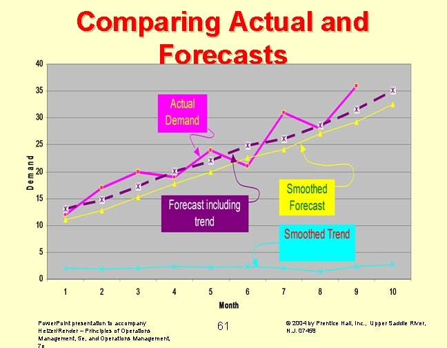
Comparing Actual and Forecasts Power. Point presentation to accompany Heizer/Render – Principles of Operations Management, 5 e, and Operations Management, 7 e 61 © 2004 by Prentice Hall, Inc. , Upper Saddle River, N. J. 07458

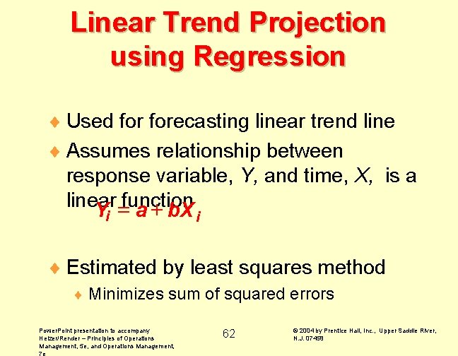
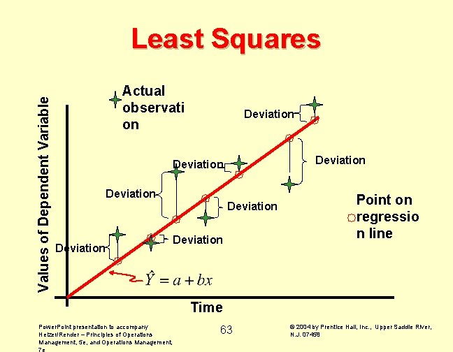
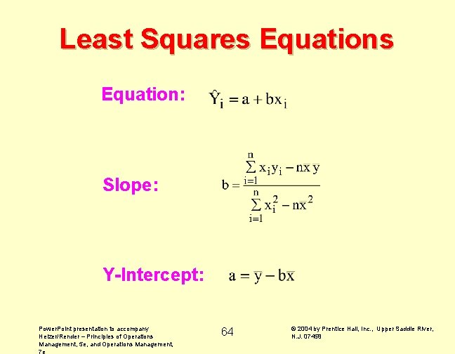
Linear Trend Projection using Regression ¨ Used forecasting linear trend line ¨ Assumes relationship between response variable, Y, and time, X, is a linear Y =function a + b. X i i ¨ Estimated by least squares method ¨ Minimizes sum of squared errors Power. Point presentation to accompany Heizer/Render – Principles of Operations Management, 5 e, and Operations Management, 7 e 62 © 2004 by Prentice Hall, Inc. , Upper Saddle River, N. J. 07458

Values of Dependent Variable Least Squares Actual observati on Deviation Deviation Point on regressio n line Time Power. Point presentation to accompany Heizer/Render – Principles of Operations Management, 5 e, and Operations Management, 7 e 63 © 2004 by Prentice Hall, Inc. , Upper Saddle River, N. J. 07458

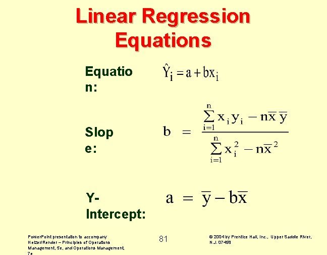
Least Squares Equation: Slope: Y-Intercept: Power. Point presentation to accompany Heizer/Render – Principles of Operations Management, 5 e, and Operations Management, 7 e 64 © 2004 by Prentice Hall, Inc. , Upper Saddle River, N. J. 07458

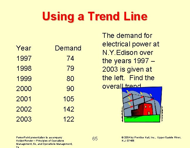
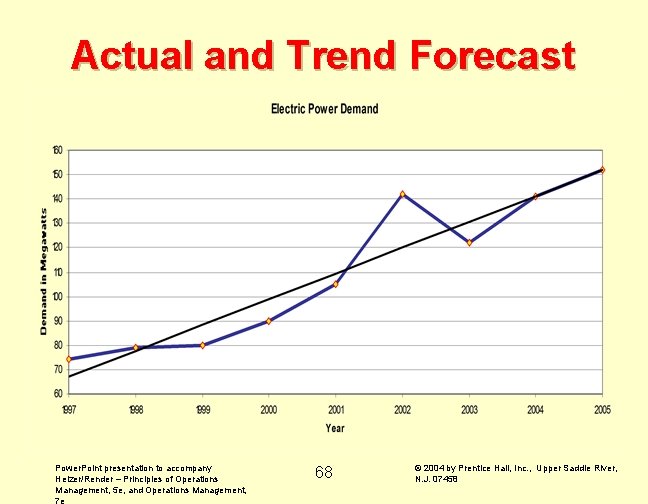
Using a Trend Line Year 1997 1998 1999 2000 2001 2002 2003 The demand for electrical power at N. Y. Edison over the years 1997 – 2003 is given at the left. Find the overall trend. Demand 74 79 80 90 105 142 122 Power. Point presentation to accompany Heizer/Render – Principles of Operations Management, 5 e, and Operations Management, 7 e 65 © 2004 by Prentice Hall, Inc. , Upper Saddle River, N. J. 07458

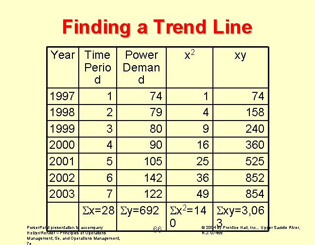
Finding a Trend Line Year Time Power x 2 xy Perio Deman d d 1997 1 74 1998 2 79 4 158 1999 3 80 9 240 2000 4 90 16 360 2001 5 105 25 525 2002 6 142 36 852 2003 7 122 49 854 x=28 y=692 x 2=14 xy=3, 06 0 3 66 Power. Point presentation to accompany Heizer/Render – Principles of Operations Management, 5 e, and Operations Management, 7 e © 2004 by Prentice Hall, Inc. , Upper Saddle River, N. J. 07458

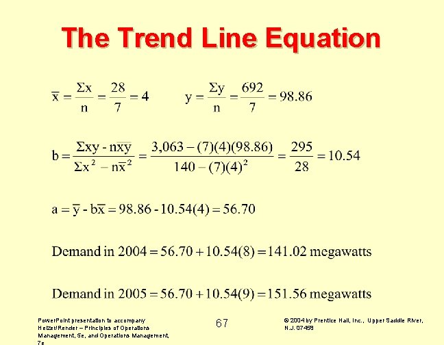
The Trend Line Equation Power. Point presentation to accompany Heizer/Render – Principles of Operations Management, 5 e, and Operations Management, 7 e 67 © 2004 by Prentice Hall, Inc. , Upper Saddle River, N. J. 07458

Actual and Trend Forecast Power. Point presentation to accompany Heizer/Render – Principles of Operations Management, 5 e, and Operations Management, 7 e 68 © 2004 by Prentice Hall, Inc. , Upper Saddle River, N. J. 07458

Seasonality Analysis Critical in capacity planning when high demand occu -electric power during winter -banks during Friday afternoons -buses subways during rush hours, -restaurants during lunch and dinner, etc. Power. Point presentation to accompany Heizer/Render – Principles of Operations Management, 5 e, and Operations Management, 7 e 69 © 2004 by Prentice Hall, Inc. , Upper Saddle River, N. J. 07458

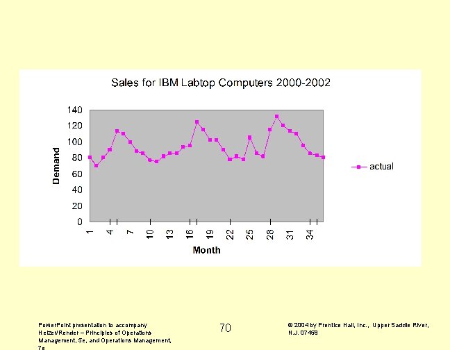
Power. Point presentation to accompany Heizer/Render – Principles of Operations Management, 5 e, and Operations Management, 7 e 70 © 2004 by Prentice Hall, Inc. , Upper Saddle River, N. J. 07458

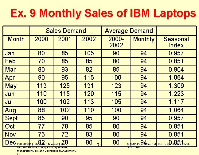
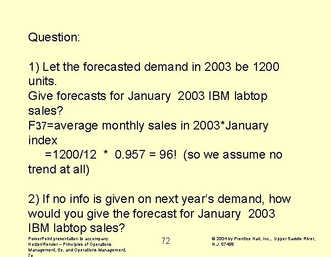
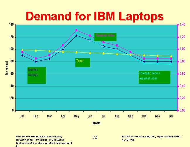
Ex. 9 Monthly Sales of IBM Laptops Month Sales Demand 2000 2001 2002 Jan 80 85 Feb 70 85 Mar 80 93 Apr 90 95 May 113 125 Jun 110 115 Jul 100 102 Aug 88 102 Sept 85 90 Oct 77 78 Nov 75 72 Dec Power. Point presentation 82 to accompany 78 Heizer/Render – Principles of Operations Management, 5 e, and Operations Management, 7 e 105 85 82 115 131 120 113 110 95 85 83 80 71 Average Demand 2000 - Monthly Seasonal 2002 Index 90 94 0. 957 80 94 0. 851 85 94 0. 904 100 94 1. 064 123 94 1. 309 115 94 1. 223 105 94 1. 117 100 94 1. 064 90 94 0. 957 80 94 0. 851 80 © 2004 by 94 0. 851 Prentice Hall, Inc. , Upper Saddle River, N. J. 07458

Question: 1) Let the forecasted demand in 2003 be 1200 units. Give forecasts for January 2003 IBM labtop sales? F 37=average monthly sales in 2003*January index =1200/12 * 0. 957 = 96! (so we assume no trend at all) 2) If no info is given on next year’s demand, how would you give the forecast for January 2003 IBM labtop sales? Power. Point presentation to accompany Heizer/Render – Principles of Operations Management, 5 e, and Operations Management, 7 e 72 © 2004 by Prentice Hall, Inc. , Upper Saddle River, N. J. 07458

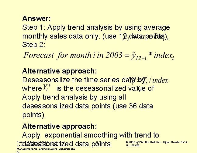
Answer: Step 1: Apply trend analysis by using average monthly sales data only. (use 12 data points), Step 2: Alternative approach: Deseasonalize the time series data by where is the deseasonalized value of Apply trend analysis by using all deseasonalized data points (use 36 data points). Alternative approach: Apply exponential smoothing with trend to 73 deseasonalized data points. Power. Point presentation to accompany Heizer/Render – Principles of Operations Management, 5 e, and Operations Management, 7 e © 2004 by Prentice Hall, Inc. , Upper Saddle River, N. J. 07458

Demand for IBM Laptops Power. Point presentation to accompany Heizer/Render – Principles of Operations Management, 5 e, and Operations Management, 7 e 74 © 2004 by Prentice Hall, Inc. , Upper Saddle River, N. J. 07458

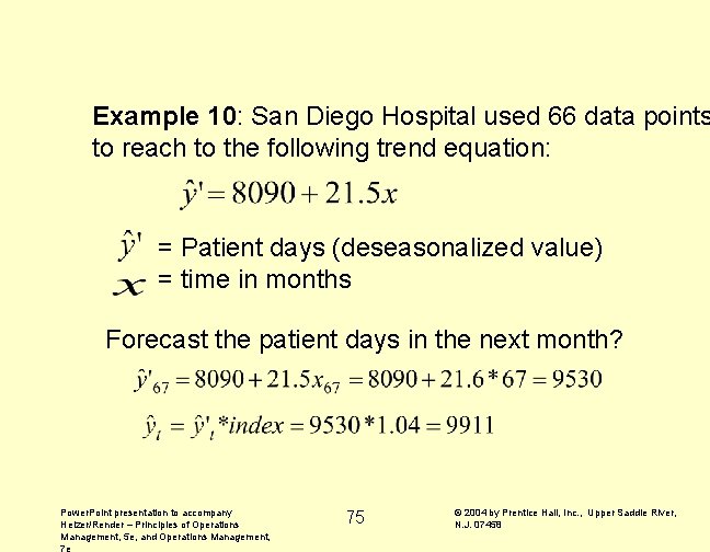
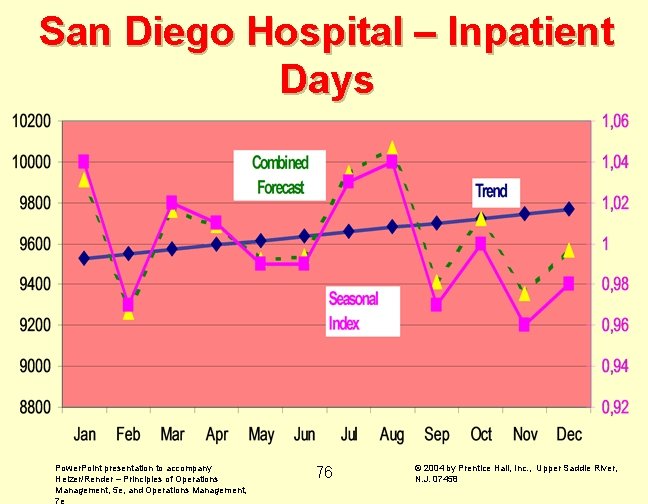
Example 10: San Diego Hospital used 66 data points to reach to the following trend equation: = Patient days (deseasonalized value) = time in months Forecast the patient days in the next month? Power. Point presentation to accompany Heizer/Render – Principles of Operations Management, 5 e, and Operations Management, 7 e 75 © 2004 by Prentice Hall, Inc. , Upper Saddle River, N. J. 07458

San Diego Hospital – Inpatient Days Power. Point presentation to accompany Heizer/Render – Principles of Operations Management, 5 e, and Operations Management, 7 e 76 © 2004 by Prentice Hall, Inc. , Upper Saddle River, N. J. 07458

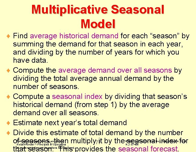
Multiplicative Seasonal Model ¨ Find average historical demand for each “season” by summing the demand for that season in each year, and dividing by the number of years for which you have data. ¨ Compute the average demand over all seasons by dividing the total average annual demand by the number of seasons. ¨ Compute a seasonal index by dividing that season’s historical demand (from step 1) by the average demand over all seasons. ¨ Estimate next year’s total demand ¨ Divide this estimate of total demand by the number of seasons, then multiply 77 it by the seasonal index for that season. This provides the seasonal forecast. Power. Point presentation to accompany Heizer/Render – Principles of Operations Management, 5 e, and Operations Management, 7 e © 2004 by Prentice Hall, Inc. , Upper Saddle River, N. J. 07458

Regression Power. Point presentation to accompany Heizer/Render – Principles of Operations Management, 5 e, and Operations Management, 7 e 78 © 2004 by Prentice Hall, Inc. , Upper Saddle River, N. J. 07458

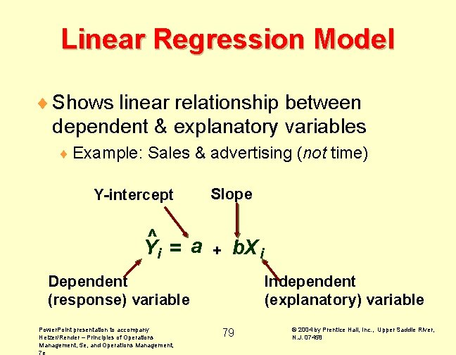
Linear Regression Model ¨ Shows linear relationship between dependent & explanatory variables ¨ Example: Sales & advertising (not time) Y-intercept Slope ^ Yi = a + b. X i Dependent (response) variable Power. Point presentation to accompany Heizer/Render – Principles of Operations Management, 5 e, and Operations Management, 7 e Independent (explanatory) variable 79 © 2004 by Prentice Hall, Inc. , Upper Saddle River, N. J. 07458

Linear Regression Equations Equatio n: Slop e: YIntercept: Power. Point presentation to accompany Heizer/Render – Principles of Operations Management, 5 e, and Operations Management, 7 e 81 © 2004 by Prentice Hall, Inc. , Upper Saddle River, N. J. 07458

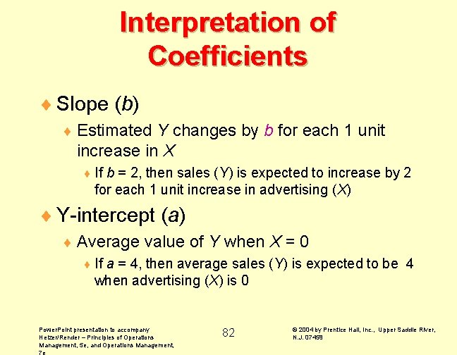
Interpretation of Coefficients ¨ Slope (b) ¨ Estimated Y changes by b for each 1 unit increase in X ¨ If b = 2, then sales (Y) is expected to increase by 2 for each 1 unit increase in advertising (X) ¨ Y-intercept (a) ¨ Average value of Y when X = 0 ¨ If a = 4, then average sales (Y) is expected to be 4 when advertising (X) is 0 Power. Point presentation to accompany Heizer/Render – Principles of Operations Management, 5 e, and Operations Management, 7 e 82 © 2004 by Prentice Hall, Inc. , Upper Saddle River, N. J. 07458

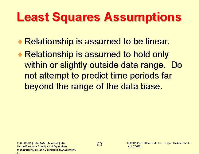
Least Squares Assumptions ¨ Relationship is assumed to be linear. ¨ Relationship is assumed to hold only within or slightly outside data range. Do not attempt to predict time periods far beyond the range of the data base. Power. Point presentation to accompany Heizer/Render – Principles of Operations Management, 5 e, and Operations Management, 7 e 83 © 2004 by Prentice Hall, Inc. , Upper Saddle River, N. J. 07458

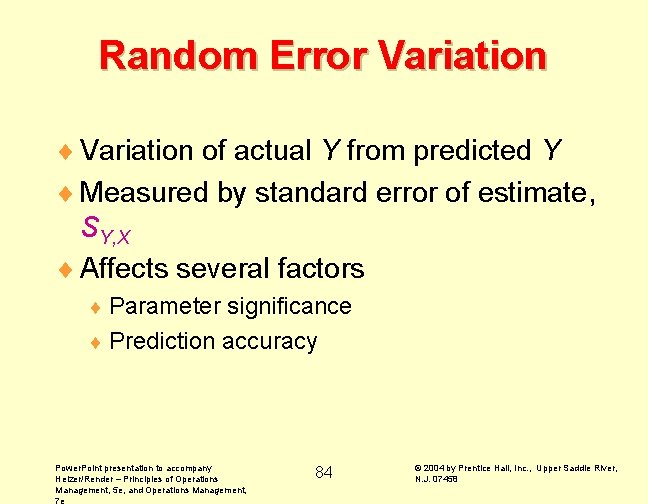
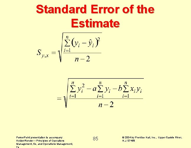
Random Error Variation ¨ Variation of actual Y from predicted Y ¨ Measured by standard error of estimate, SY, X ¨ Affects several factors ¨ Parameter significance ¨ Prediction accuracy Power. Point presentation to accompany Heizer/Render – Principles of Operations Management, 5 e, and Operations Management, 7 e 84 © 2004 by Prentice Hall, Inc. , Upper Saddle River, N. J. 07458

Standard Error of the Estimate Power. Point presentation to accompany Heizer/Render – Principles of Operations Management, 5 e, and Operations Management, 7 e 85 © 2004 by Prentice Hall, Inc. , Upper Saddle River, N. J. 07458

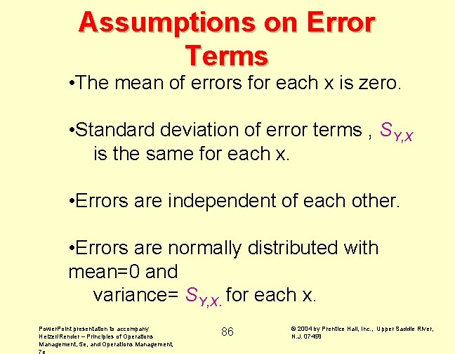
Assumptions on Error Terms • The mean of errors for each x is zero. • Standard deviation of error terms , SY, X is the same for each x. • Errors are independent of each other. • Errors are normally distributed with mean=0 and variance= SY, X. for each x. Power. Point presentation to accompany Heizer/Render – Principles of Operations Management, 5 e, and Operations Management, 7 e 86 © 2004 by Prentice Hall, Inc. , Upper Saddle River, N. J. 07458

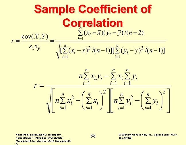
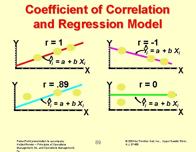
Correlation ¨ Answers: ‘how strong is the linear relationship between the variables? ’ ¨ Correlation coefficient, r ¨ Values range from -1 to +1 ¨ Measures degree of association ¨ Used mainly for understanding Power. Point presentation to accompany Heizer/Render – Principles of Operations Management, 5 e, and Operations Management, 7 e 87 © 2004 by Prentice Hall, Inc. , Upper Saddle River, N. J. 07458

Sample Coefficient of Correlation Power. Point presentation to accompany Heizer/Render – Principles of Operations Management, 5 e, and Operations Management, 7 e 88 © 2004 by Prentice Hall, Inc. , Upper Saddle River, N. J. 07458

Coefficient of Correlation and Regression Model Y r=1 Y ^i = a + b Xi Y r = -1 ^i = a + b Xi Y X r =. 89 ^i = a + b Xi Y Power. Point presentation to accompany Heizer/Render – Principles of Operations Management, 5 e, and Operations Management, 7 e Y r=0 ^i = a + b Xi Y X 89 X © 2004 by Prentice Hall, Inc. , Upper Saddle River, N. J. 07458

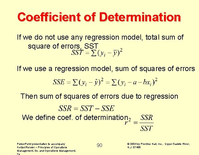
Coefficient of Determination If we do not use any regression model, total sum of square of errors, SST If we use a regression model, sum of squares of errors Then sum of squares of errors due to regression We define coef. of determination Power. Point presentation to accompany Heizer/Render – Principles of Operations Management, 5 e, and Operations Management, 7 e 90 © 2004 by Prentice Hall, Inc. , Upper Saddle River, N. J. 07458

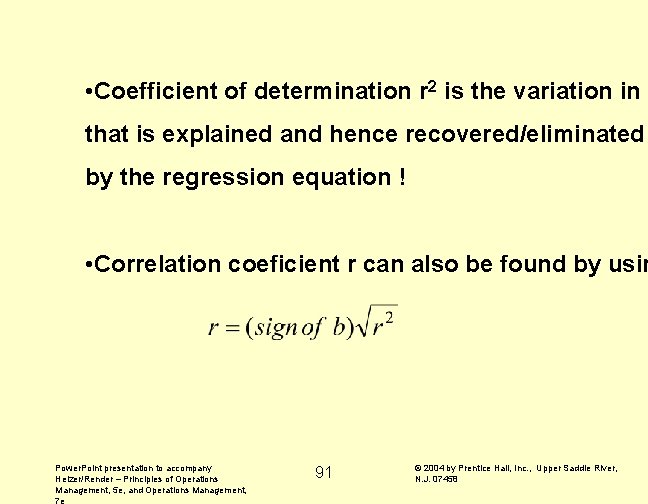
• Coefficient of determination r 2 is the variation in y that is explained and hence recovered/eliminated by the regression equation ! • Correlation coeficient r can also be found by usin Power. Point presentation to accompany Heizer/Render – Principles of Operations Management, 5 e, and Operations Management, 7 e 91 © 2004 by Prentice Hall, Inc. , Upper Saddle River, N. J. 07458

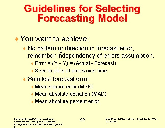
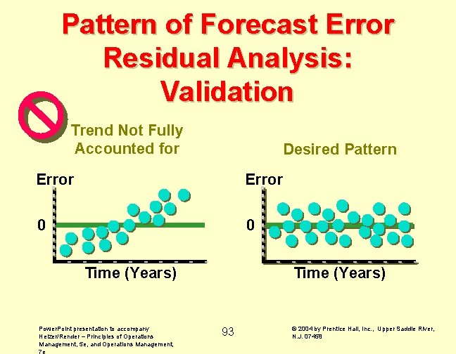
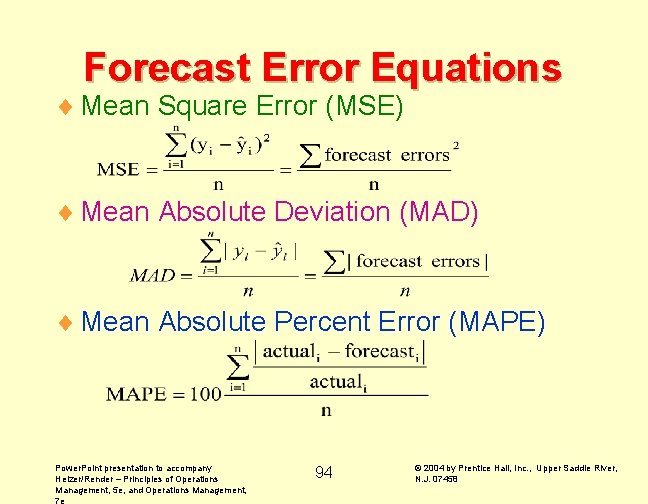
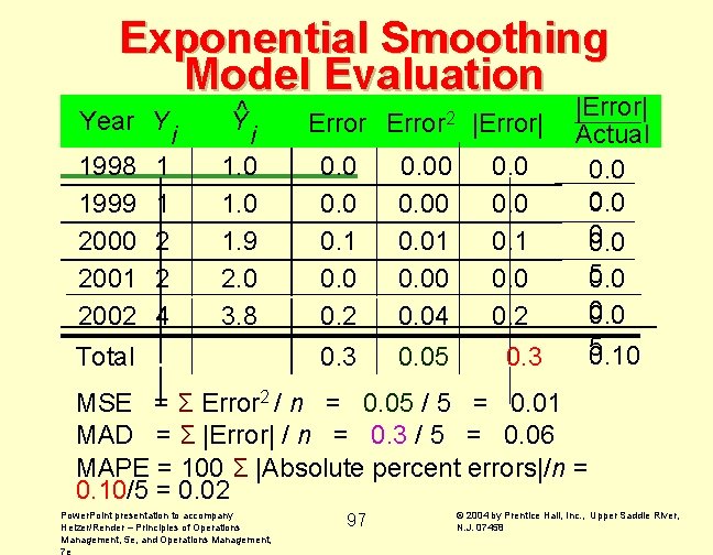
Guidelines for Selecting Forecasting Model ¨ You want to achieve: ¨ No pattern or direction in forecast error, ^ remember independency of errors assumption. ¨ Error = (Yi - Yi) = (Actual - Forecast) ¨ Seen in plots of errors over time ¨ Smallest forecast error ¨ Mean square error (MSE) ¨ Mean absolute deviation (MAD) ¨ Mean absolute percent error Power. Point presentation to accompany Heizer/Render – Principles of Operations Management, 5 e, and Operations Management, 7 e 92 © 2004 by Prentice Hall, Inc. , Upper Saddle River, N. J. 07458

Pattern of Forecast Error Residual Analysis: Validation Trend Not Fully Accounted for Desired Pattern Error 0 0 Time (Years) Power. Point presentation to accompany Heizer/Render – Principles of Operations Management, 5 e, and Operations Management, 7 e Time (Years) 93 © 2004 by Prentice Hall, Inc. , Upper Saddle River, N. J. 07458

Forecast Error Equations ¨ Mean Square Error (MSE) ¨ Mean Absolute Deviation (MAD) ¨ Mean Absolute Percent Error (MAPE) Power. Point presentation to accompany Heizer/Render – Principles of Operations Management, 5 e, and Operations Management, 7 e 94 © 2004 by Prentice Hall, Inc. , Upper Saddle River, N. J. 07458

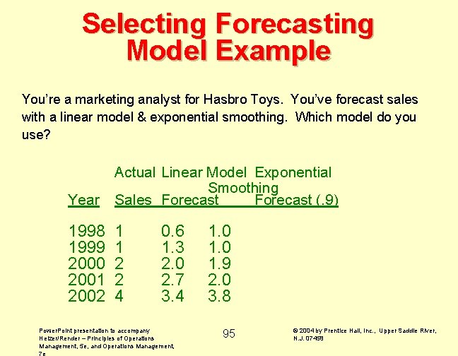
Selecting Forecasting Model Example You’re a marketing analyst for Hasbro Toys. You’ve forecast sales with a linear model & exponential smoothing. Which model do you use? Year Actual Linear Model Exponential Smoothing Sales Forecast (. 9) 1998 1999 2000 2001 2002 1 1 2 2 4 0. 6 1. 3 2. 0 2. 7 3. 4 Power. Point presentation to accompany Heizer/Render – Principles of Operations Management, 5 e, and Operations Management, 7 e 1. 0 1. 9 2. 0 3. 8 95 © 2004 by Prentice Hall, Inc. , Upper Saddle River, N. J. 07458

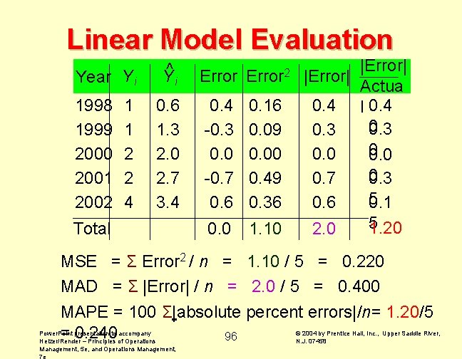
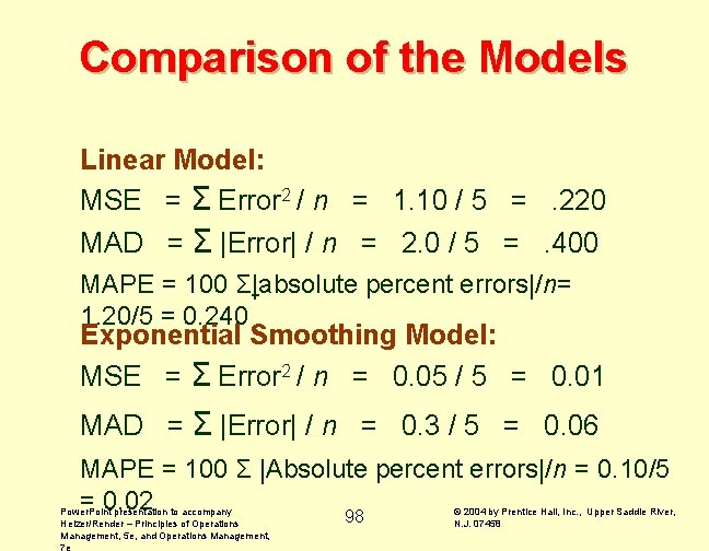
Linear Model Evaluation Year Y i 1998 1999 2000 2001 2002 1 1 2 2 4 Y^ i 0. 6 1. 3 2. 0 2. 7 3. 4 Total Error 2 |Error| 0. 4 -0. 3 0. 0 -0. 7 0. 6 0. 16 0. 09 0. 00 0. 49 0. 36 0. 4 0. 3 0. 0 0. 7 0. 6 0. 0 1. 10 2. 0 |Error| Actua l 0. 4 0. 3 0 0. 3 5 0. 1 5 1. 20 MSE = Σ Error 2 / n = 1. 10 / 5 = 0. 220 MAD = Σ |Error| / n = 2. 0 / 5 = 0. 400 MAPE = 100 Σ|absolute percent errors|/n= 1. 20/5 = 0. 240 96 Power. Point presentation to accompany Heizer/Render – Principles of Operations Management, 5 e, and Operations Management, 7 e © 2004 by Prentice Hall, Inc. , Upper Saddle River, N. J. 07458

Exponential Smoothing Model Evaluation Year Y 1998 1999 2000 2001 2002 1 1 2 2 4 i Y^ i 1. 0 1. 9 2. 0 3. 8 Total Error 2 |Error| 0. 0 0. 1 0. 0 0. 2 0. 00 0. 01 0. 00 0. 04 0. 3 0. 05 0. 0 0. 1 0. 0 0. 2 0. 3 |Error| Actual 0. 0 0 0. 0 5 0. 10 MSE = Σ Error 2 / n = 0. 05 / 5 = 0. 01 MAD = Σ |Error| / n = 0. 3 / 5 = 0. 06 MAPE = 100 Σ |Absolute percent errors|/n = 0. 10/5 = 0. 02 Power. Point presentation to accompany Heizer/Render – Principles of Operations Management, 5 e, and Operations Management, 7 e 97 © 2004 by Prentice Hall, Inc. , Upper Saddle River, N. J. 07458

Comparison of the Models Linear Model: MSE = Σ Error 2 / n = 1. 10 / 5 =. 220 MAD = Σ |Error| / n = 2. 0 / 5 =. 400 MAPE = 100 Σ|absolute percent errors|/n= 1. 20/5 = 0. 240 Exponential Smoothing Model: MSE = Σ Error 2 / n = 0. 05 / 5 = 0. 01 MAD = Σ |Error| / n = 0. 3 / 5 = 0. 06 MAPE = 100 Σ |Absolute percent errors|/n = 0. 10/5 = 0. 02 98 Power. Point presentation to accompany Heizer/Render – Principles of Operations Management, 5 e, and Operations Management, 7 e © 2004 by Prentice Hall, Inc. , Upper Saddle River, N. J. 07458

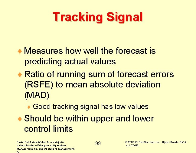
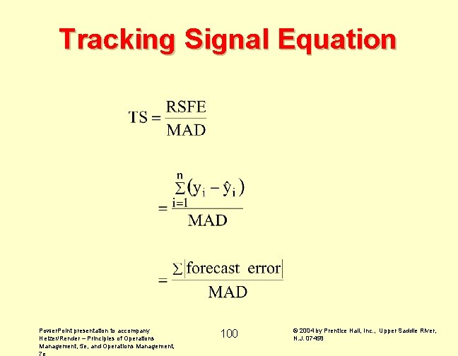
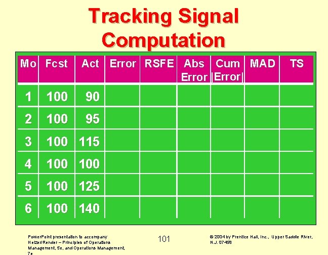
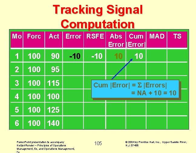
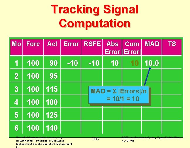
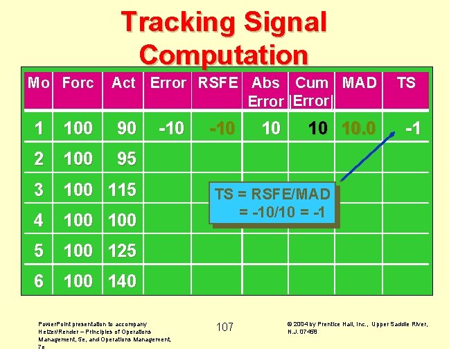
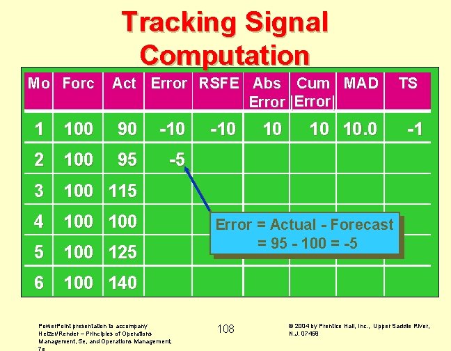
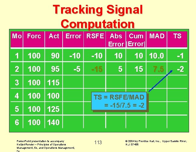
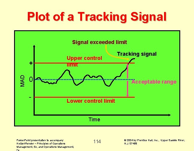
Tracking Signal ¨ Measures how well the forecast is predicting actual values ¨ Ratio of running sum of forecast errors (RSFE) to mean absolute deviation (MAD) ¨ Good tracking signal has low values ¨ Should be within upper and lower control limits Power. Point presentation to accompany Heizer/Render – Principles of Operations Management, 5 e, and Operations Management, 7 e 99 © 2004 by Prentice Hall, Inc. , Upper Saddle River, N. J. 07458

Tracking Signal Equation Power. Point presentation to accompany Heizer/Render – Principles of Operations Management, 5 e, and Operations Management, 7 e 100 © 2004 by Prentice Hall, Inc. , Upper Saddle River, N. J. 07458

Tracking Signal Computation Mo Fcst Act Error RSFE Abs Cum MAD Error |Error| 1 100 90 2 100 95 3 100 115 4 100 5 100 125 6 100 140 Power. Point presentation to accompany Heizer/Render – Principles of Operations Management, 5 e, and Operations Management, 7 e 101 TS © 2004 by Prentice Hall, Inc. , Upper Saddle River, N. J. 07458

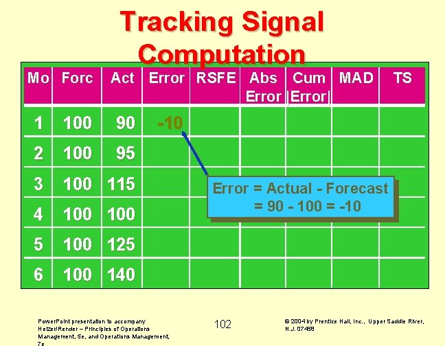
Mo Forc Tracking Signal Computation Act Error RSFE Abs Cum MAD Error |Error| 1 100 90 2 100 95 3 100 115 4 100 5 100 125 6 100 140 TS -10 Power. Point presentation to accompany Heizer/Render – Principles of Operations Management, 5 e, and Operations Management, 7 e Error = Actual - Forecast = 90 - 100 = -10 102 © 2004 by Prentice Hall, Inc. , Upper Saddle River, N. J. 07458

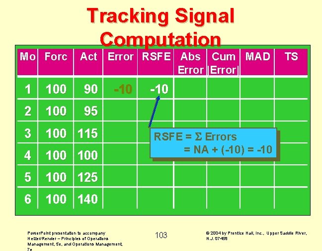
Mo Forc Tracking Signal Computation Act Error RSFE Abs Cum MAD Error |Error| 1 100 90 2 100 95 3 100 115 4 100 5 100 125 6 100 140 -10 Power. Point presentation to accompany Heizer/Render – Principles of Operations Management, 5 e, and Operations Management, 7 e TS -10 RSFE = Errors = NA + (-10) = -10 103 © 2004 by Prentice Hall, Inc. , Upper Saddle River, N. J. 07458

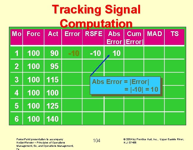
Mo Forc Tracking Signal Computation Act Error RSFE Abs Cum MAD Error |Error| 1 100 90 2 100 95 3 100 115 4 100 5 100 125 6 100 140 -10 Power. Point presentation to accompany Heizer/Render – Principles of Operations Management, 5 e, and Operations Management, 7 e -10 TS 10 Abs Error = |Error| = |-10| = 10 104 © 2004 by Prentice Hall, Inc. , Upper Saddle River, N. J. 07458

Tracking Signal Computation Mo Forc Act Error RSFE Abs Cum MAD Error |Error| 1 100 90 2 100 95 3 100 115 4 100 5 100 125 6 100 140 -10 Power. Point presentation to accompany Heizer/Render – Principles of Operations Management, 5 e, and Operations Management, 7 e -10 10 TS 10 Cum |Error| = |Errors| = NA + 10 = 10 105 © 2004 by Prentice Hall, Inc. , Upper Saddle River, N. J. 07458

Tracking Signal Computation Mo Forc Act Error RSFE Abs Cum MAD Error |Error| 1 100 90 2 100 95 3 100 115 4 100 5 100 125 6 100 140 -10 Power. Point presentation to accompany Heizer/Render – Principles of Operations Management, 5 e, and Operations Management, 7 e -10 10 TS 10 10. 0 MAD = |Errors|/n = 10/1 = 10 106 © 2004 by Prentice Hall, Inc. , Upper Saddle River, N. J. 07458

Tracking Signal Computation Mo Forc Act Error RSFE Abs Cum MAD Error |Error| 1 100 90 2 100 95 3 100 115 4 100 5 100 125 6 100 140 -10 Power. Point presentation to accompany Heizer/Render – Principles of Operations Management, 5 e, and Operations Management, 7 e -10 10. 0 TS -1 TS = RSFE/MAD = -10/10 = -1 107 © 2004 by Prentice Hall, Inc. , Upper Saddle River, N. J. 07458

Tracking Signal Computation Mo Forc Act Error RSFE Abs Cum MAD Error |Error| 1 100 90 -10 2 100 95 -5 3 100 115 4 100 5 100 125 6 100 140 Power. Point presentation to accompany Heizer/Render – Principles of Operations Management, 5 e, and Operations Management, 7 e -10 10. 0 TS -1 Error = Actual - Forecast = 95 - 100 = -5 108 © 2004 by Prentice Hall, Inc. , Upper Saddle River, N. J. 07458

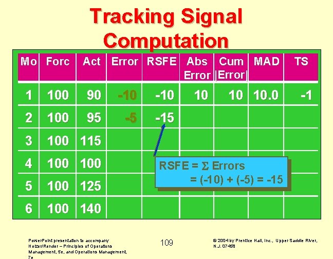
Tracking Signal Computation Mo Forc Act Error RSFE Abs Cum MAD Error |Error| 1 100 90 -10 2 100 95 -5 -15 3 100 115 4 100 5 100 125 6 100 140 Power. Point presentation to accompany Heizer/Render – Principles of Operations Management, 5 e, and Operations Management, 7 e 10 10 10. 0 TS -1 RSFE = Errors = (-10) + (-5) = -15 109 © 2004 by Prentice Hall, Inc. , Upper Saddle River, N. J. 07458

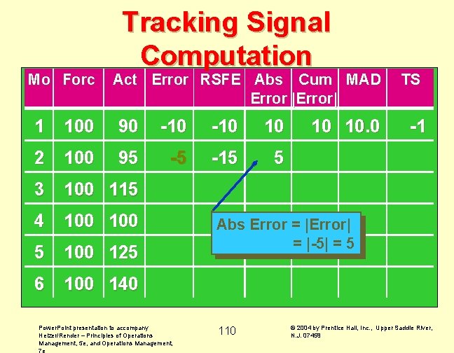
Mo Forc Tracking Signal Computation Act Error RSFE Abs Cum MAD Error |Error| 1 100 90 -10 10 2 100 95 -5 -15 5 3 100 115 4 100 5 100 125 6 100 140 Power. Point presentation to accompany Heizer/Render – Principles of Operations Management, 5 e, and Operations Management, 7 e 10 10. 0 TS -1 Abs Error = |Error| = |-5| = 5 110 © 2004 by Prentice Hall, Inc. , Upper Saddle River, N. J. 07458

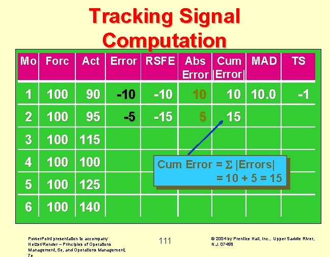
Tracking Signal Computation Mo Forc Act Error RSFE Abs Cum MAD Error |Error| 1 100 90 -10 10 2 100 95 -5 -15 5 3 100 115 4 100 5 100 125 6 100 140 Power. Point presentation to accompany Heizer/Render – Principles of Operations Management, 5 e, and Operations Management, 7 e 10 10. 0 TS -1 15 Cum Error = |Errors| = 10 + 5 = 15 111 © 2004 by Prentice Hall, Inc. , Upper Saddle River, N. J. 07458

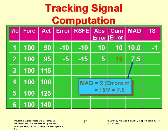
Tracking Signal Computation Mo Forc Act Error RSFE Abs Cum MAD Error |Error| 1 100 90 -10 10 2 100 95 -5 -15 5 3 100 115 4 100 5 100 125 6 100 140 Power. Point presentation to accompany Heizer/Render – Principles of Operations Management, 5 e, and Operations Management, 7 e 10 10. 0 15 TS -1 7. 5 MAD = |Errors|/n = 15/2 = 7. 5 112 © 2004 by Prentice Hall, Inc. , Upper Saddle River, N. J. 07458

Tracking Signal Computation Mo Forc Act Error RSFE Abs Cum MAD Error |Error| 1 100 90 -10 10 2 100 95 -5 -15 5 3 100 115 4 100 5 100 125 6 100 140 Power. Point presentation to accompany Heizer/Render – Principles of Operations Management, 5 e, and Operations Management, 7 e TS 10 10. 0 -1 15 -2 7. 5 TS = RSFE/MAD = -15/7. 5 = -2 113 © 2004 by Prentice Hall, Inc. , Upper Saddle River, N. J. 07458

Plot of a Tracking Signal exceeded limit MAD + Upper control limit 0 - Tracking signal Acceptable range Lower control limit Time Power. Point presentation to accompany Heizer/Render – Principles of Operations Management, 5 e, and Operations Management, 7 e 114 © 2004 by Prentice Hall, Inc. , Upper Saddle River, N. J. 07458

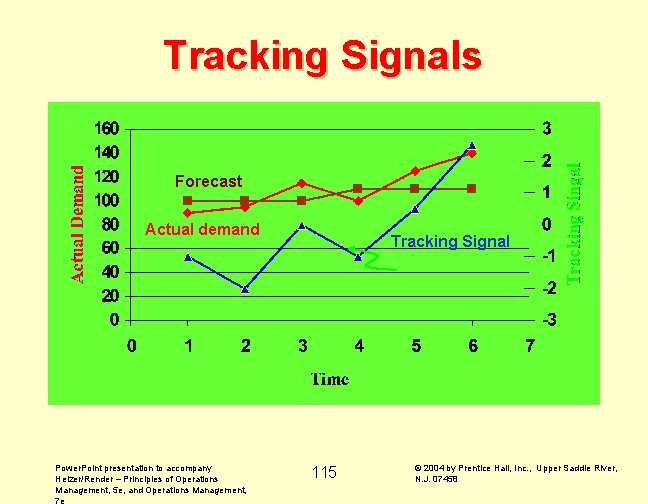
Tracking Signals Forecast Actual demand Power. Point presentation to accompany Heizer/Render – Principles of Operations Management, 5 e, and Operations Management, 7 e Tracking Signal 115 © 2004 by Prentice Hall, Inc. , Upper Saddle River, N. J. 07458

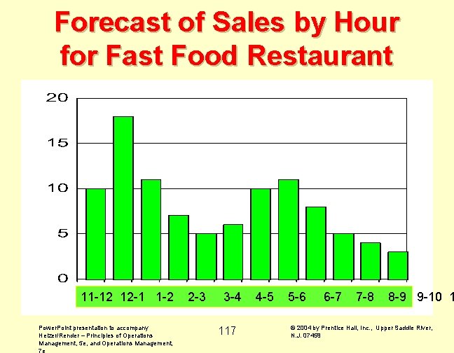
Forecasting in the Service Sector ¨ Presents unusual challenges ¨ special need for short term records ¨ needs differ greatly as function of industry and product ¨ issues of holidays and calendar ¨ unusual events Power. Point presentation to accompany Heizer/Render – Principles of Operations Management, 5 e, and Operations Management, 7 e 116 © 2004 by Prentice Hall, Inc. , Upper Saddle River, N. J. 07458

Forecast of Sales by Hour for Fast Food Restaurant 11 -12 12 -1 1 -2 Power. Point presentation to accompany Heizer/Render – Principles of Operations Management, 5 e, and Operations Management, 7 e 2 -3 3 -4 117 4 -5 5 -6 6 -7 7 -8 8 -9 9 -10 1 © 2004 by Prentice Hall, Inc. , Upper Saddle River, N. J. 07458