Quality Control Dr Everette S Gardner Jr 8

Quality Control Dr. Everette S. Gardner, Jr. 8 -

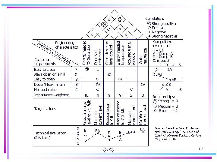
Correlation: Strong positive Positive x Negative * Strong negative Competitive evaluation x = Us A = Comp. A B = Comp. B (5 is best) 1 2 3 4 5 x AB A x. B x A B x x x Acoustic trans. , window Water resistance 10 6 6 9 2 3 Maintain current level B x. A BA x 7 5 3 3 2 Importance weighting Target values Technical evaluation (5 is best) Energy needed to open door Easy to close Stays open on a hill Easy to open Doesn’t leak in rain No road noise Reduce energy to 7. 5 ft/lb er Check force on level ground tom Reduce force to 9 lb. Customer requirements Door seal resistance to cu s Maintain current level ce Engineering characteristics Energy needed to close door Im po rta n x Reduce energy level to 7. 5 ft/lb x 5 4 3 2 1 B A x Quality B x A Relationships: Strong = 9 Medium = 3 Small = 1 Source: Based on John R. Hauser and Don Clausing, “The House of Quality, ” Harvard Business Review, May-June 1988. 8 -2

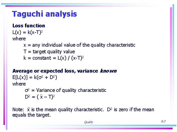
Taguchi analysis Loss function L(x) = k(x-T)2 where x = any individual value of the quality characteristic T = target quality value k = constant = L(x) / (x-T)2 Average or expected loss, variance known E[L(x)] = k(σ2 + D 2) where σ2 = Variance of quality characteristic D 2 = ( x – T)2 Note: x is the mean quality characteristic. D 2 is zero if the mean equals the target. Quality 8 -3

Taguchi analysis (cont. ) Average or expected loss, variance unkown E[L(x)] = k[Σ ( x – T)2 / n] When smaller is better (e. g. , percent of impurities) L(x) = kx 2 When larger is better (e. g. , product life) L(x) = k (1/x 2) Quality 8 -4

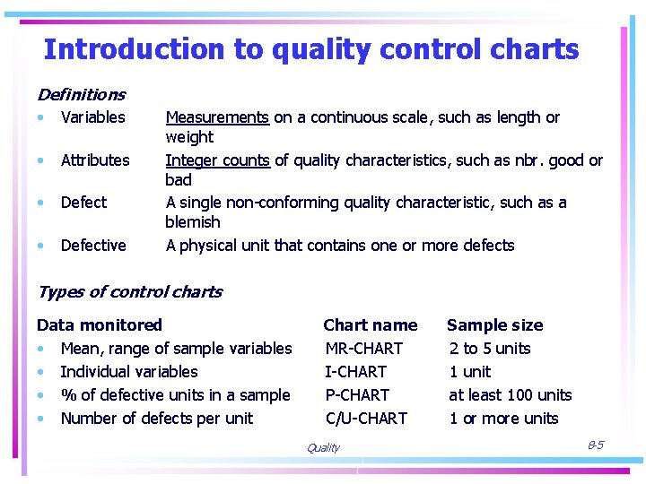
Introduction to quality control charts Definitions • Variables • Attributes • Defective Measurements on a continuous scale, such as length or weight Integer counts of quality characteristics, such as nbr. good or bad A single non-conforming quality characteristic, such as a blemish A physical unit that contains one or more defects Types of control charts Data monitored • Mean, range of sample variables • Individual variables • % of defective units in a sample • Number of defects per unit Chart name MR-CHART I-CHART P-CHART C/U-CHART Quality Sample size 2 to 5 units 1 unit at least 100 units 1 or more units 8 -5

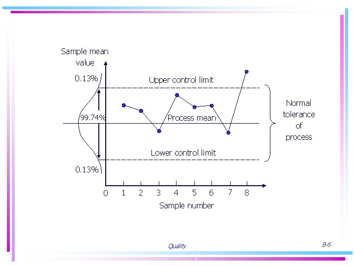
Sample mean value 0. 13% Upper control limit 99. 74% Normal tolerance of process Process mean Lower control limit 0. 13% 0 1 2 3 4 5 6 7 8 Sample number Quality 8 -6

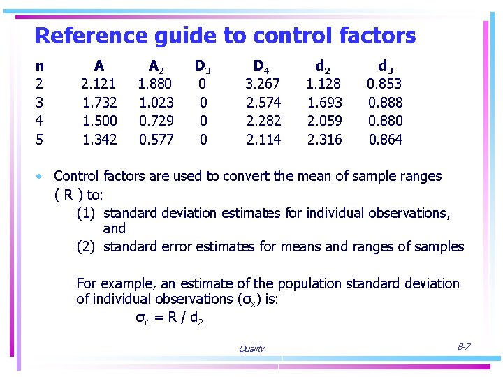
Reference guide to control factors n 2 3 4 5 A 2. 121 1. 732 1. 500 1. 342 A 2 1. 880 1. 023 0. 729 0. 577 D 3 0 0 D 4 3. 267 2. 574 2. 282 2. 114 d 2 1. 128 1. 693 2. 059 2. 316 d 3 0. 853 0. 888 0. 880 0. 864 • Control factors are used to convert the mean of sample ranges ( R ) to: (1) standard deviation estimates for individual observations, and (2) standard error estimates for means and ranges of samples For example, an estimate of the population standard deviation of individual observations (σx) is: σx = R / d 2 Quality 8 -7

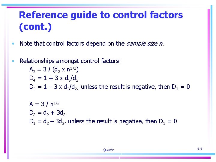
Reference guide to control factors (cont. ) • Note that control factors depend on the sample size n. • Relationships amongst control factors: A 2 = 3 / (d 2 x n 1/2) D 4 = 1 + 3 x d 3/d 2 D 3 = 1 – 3 x d 3/d 2, unless the result is negative, then D 3 = 0 A = 3 / n 1/2 D 2 = d 2 + 3 d 3 D 1 = d 2 – 3 d 3, unless the result is negative, then D 1 = 0 Quality 8 -8

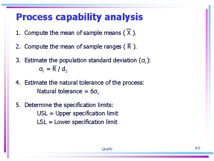
Process capability analysis 1. Compute the mean of sample means ( X ). 2. Compute the mean of sample ranges ( R ). 3. Estimate the population standard deviation (σx): σx = R / d 2 4. Estimate the natural tolerance of the process: Natural tolerance = 6σx 5. Determine the specification limits: USL = Upper specification limit LSL = Lower specification limit Quality 8 -9

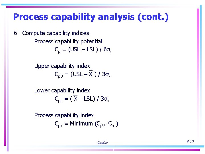
Process capability analysis (cont. ) 6. Compute capability indices: Process capability potential Cp = (USL – LSL) / 6σx Upper capability index Cp. U = (USL – X ) / 3σx Lower capability index Cp. L = ( X – LSL) / 3σx Process capability index Cpk = Minimum (Cp. U, Cp. L) Quality 8 -10

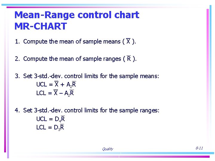
Mean-Range control chart MR-CHART 1. Compute the mean of sample means ( X ). 2. Compute the mean of sample ranges ( R ). 3. Set 3 -std. -dev. control limits for the sample means: UCL = X + A 2 R LCL = X – A 2 R 4. Set 3 -std. -dev. control limits for the sample ranges: UCL = D 4 R LCL = D 3 R Quality 8 -11

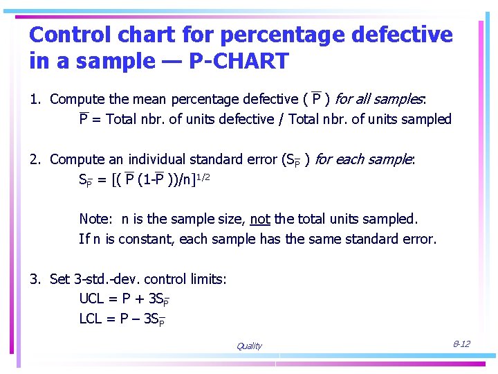
Control chart for percentage defective in a sample — P-CHART 1. Compute the mean percentage defective ( P ) for all samples: P = Total nbr. of units defective / Total nbr. of units sampled 2. Compute an individual standard error (SP ) for each sample: SP = [( P (1 -P ))/n]1/2 Note: n is the sample size, not the total units sampled. If n is constant, each sample has the same standard error. 3. Set 3 -std. -dev. control limits: UCL = P + 3 SP LCL = P – 3 SP Quality 8 -12

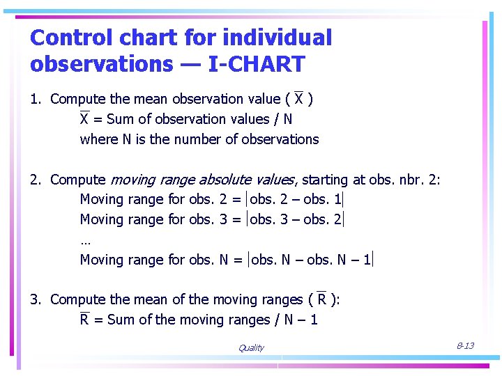
Control chart for individual observations — I-CHART 1. Compute the mean observation value ( X ) X = Sum of observation values / N where N is the number of observations 2. Compute moving range absolute values, starting at obs. nbr. 2: Moving range for obs. 2 = obs. 2 – obs. 1 Moving range for obs. 3 = obs. 3 – obs. 2 … Moving range for obs. N = obs. N – 1 3. Compute the mean of the moving ranges ( R ): R = Sum of the moving ranges / N – 1 Quality 8 -13

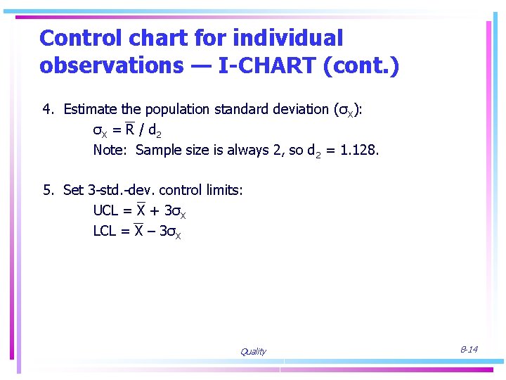
Control chart for individual observations — I-CHART (cont. ) 4. Estimate the population standard deviation (σX): σX = R / d 2 Note: Sample size is always 2, so d 2 = 1. 128. 5. Set 3 -std. -dev. control limits: UCL = X + 3σX LCL = X – 3σX Quality 8 -14

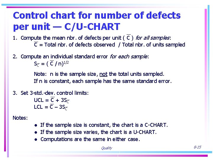
Control chart for number of defects per unit — C/U-CHART 1. Compute the mean nbr. of defects per unit ( C ) for all samples: C = Total nbr. of defects observed / Total nbr. of units sampled 2. Compute an individual standard error for each sample: SC = ( C / n)1/2 Note: n is the sample size, not the total units sampled. If n is constant, each sample has the same standard error. 3. Set 3 -std. -dev. control limits: UCL = C + 3 SC LCL = C – 3 SC Notes: ● If the sample size is constant, the chart is a C-CHART. ● If the sample size varies, the chart is a U-CHART. ● Computations are the same in either case. Quality 8 -15

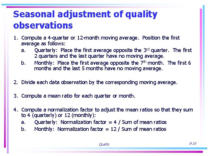
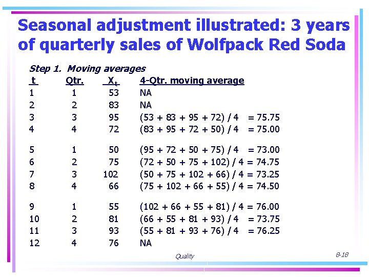
Seasonal adjustment of quality observations 1. Compute a 4 -quarter or 12 -month moving average. Position the first average as follows: a. Quarterly: Place the first average opposite the 3 rd quarter. The first 2 quarters and the last quarter have no moving average. b. Monthly: Place the first average opposite the 7 th month. The first 6 months and the last 5 months have no moving average. 2. Divide each data observation by the corresponding moving average. 3. Compute a mean ratio for each quarter or month. 4. Compute a normalization factor to adjust the mean ratios so that they sum to 4 (quarterly) or 12 (monthly): a. Quarterly: Normalization factor = 4 / Sum of mean ratios b. Monthly: Normalization factor = 12 / Sum of mean ratios Quality 8 -16

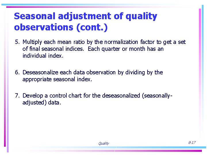
Seasonal adjustment of quality observations (cont. ) 5. Multiply each mean ratio by the normalization factor to get a set of final seasonal indices. Each quarter or month has an individual index. 6. Deseasonalize each data observation by dividing by the appropriate seasonal index. 7. Develop a control chart for the deseasonalized (seasonallyadjusted) data. Quality 8 -17

Seasonal adjustment illustrated: 3 years of quarterly sales of Wolfpack Red Soda Step 1. Moving averages t 1 2 3 4 Qtr. 1 2 3 4 Xt 53 83 95 72 5 6 7 8 1 2 3 4 50 75 102 66 9 10 11 12 1 2 3 4 55 81 93 76 4 -Qtr. moving average NA NA (53 + 83 + 95 + 72) / 4 = 75. 75 (83 + 95 + 72 + 50) / 4 = 75. 00 (95 (72 (50 (75 + + 72 + 50 + 75) / 4 50 + 75 + 102) / 4 75 + 102 + 66) / 4 102 + 66 + 55) / 4 = 73. 00 = 74. 75 = 73. 25 = 74. 50 (102 + 66 + 55 + 81) / 4 = 76. 00 (66 + 55 + 81 + 93) / 4 = 73. 75 (55 + 81 + 93 + 76) / 4 = 76. 25 NA Quality 8 -18

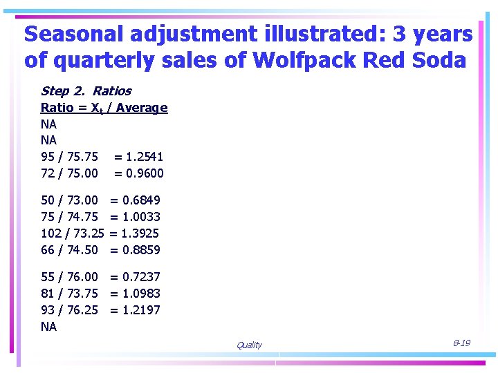
Seasonal adjustment illustrated: 3 years of quarterly sales of Wolfpack Red Soda Step 2. Ratios Ratio = Xt / Average NA NA 95 / 75. 75 = 1. 2541 72 / 75. 00 = 0. 9600 50 / 73. 00 75 / 74. 75 102 / 73. 25 66 / 74. 50 = 0. 6849 = 1. 0033 = 1. 3925 = 0. 8859 55 / 76. 00 = 0. 7237 81 / 73. 75 = 1. 0983 93 / 76. 25 = 1. 2197 NA Quality 8 -19

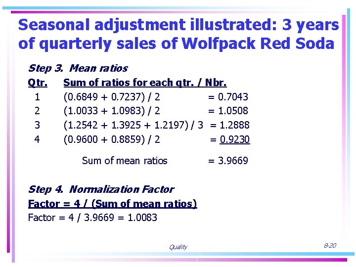
Seasonal adjustment illustrated: 3 years of quarterly sales of Wolfpack Red Soda Step 3. Mean ratios Qtr. 1 2 3 4 Sum of ratios for each qtr. / Nbr. (0. 6849 + 0. 7237) / 2 = 0. 7043 (1. 0033 + 1. 0983) / 2 = 1. 0508 (1. 2542 + 1. 3925 + 1. 2197) / 3 = 1. 2888 (0. 9600 + 0. 8859) / 2 = 0. 9230 Sum of mean ratios = 3. 9669 Step 4. Normalization Factor = 4 / (Sum of mean ratios) Factor = 4 / 3. 9669 = 1. 0083 Quality 8 -20

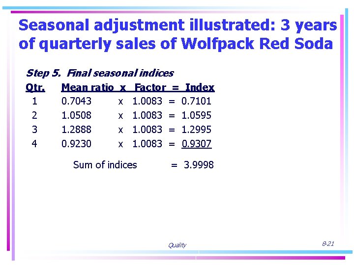
Seasonal adjustment illustrated: 3 years of quarterly sales of Wolfpack Red Soda Step 5. Final seasonal indices Qtr. 1 2 3 4 Mean ratio 0. 7043 1. 0508 1. 2888 0. 9230 x x x Factor = Index 1. 0083 = 0. 7101 1. 0083 = 1. 0595 1. 0083 = 1. 2995 1. 0083 = 0. 9307 Sum of indices = 3. 9998 Quality 8 -21

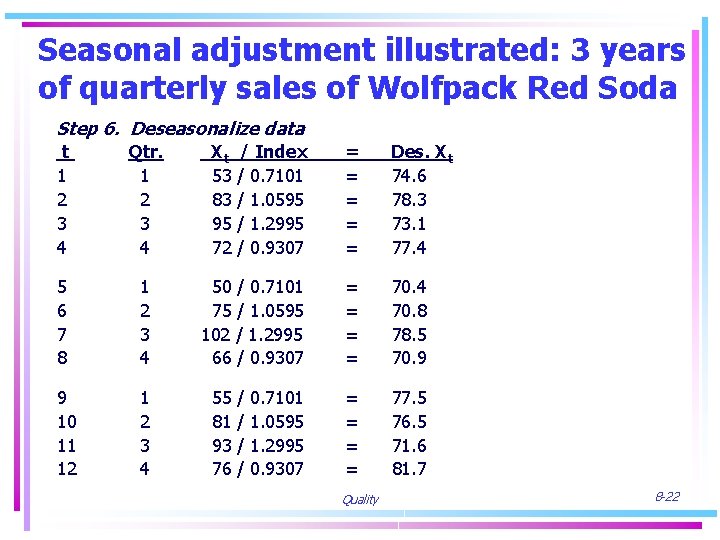
Seasonal adjustment illustrated: 3 years of quarterly sales of Wolfpack Red Soda Step 6. Deseasonalize data t 1 2 3 4 Qtr. 1 2 3 4 5 6 7 8 1 2 3 4 9 10 11 12 1 2 3 4 Xt 53 83 95 72 / Index / 0. 7101 / 1. 0595 / 1. 2995 / 0. 9307 = = = Des. Xt 74. 6 78. 3 73. 1 77. 4 50 / 0. 7101 75 / 1. 0595 102 / 1. 2995 66 / 0. 9307 = = 70. 4 70. 8 78. 5 70. 9 = = 77. 5 76. 5 71. 6 81. 7 55 81 93 76 / / 0. 7101 1. 0595 1. 2995 0. 9307 Quality 8 -22

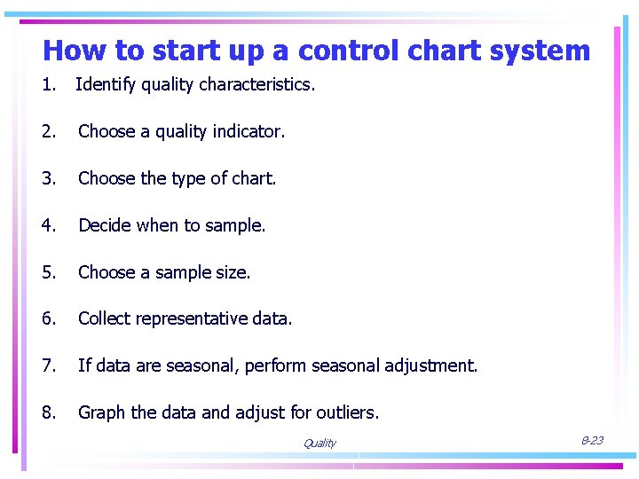
How to start up a control chart system 1. Identify quality characteristics. 2. Choose a quality indicator. 3. Choose the type of chart. 4. Decide when to sample. 5. Choose a sample size. 6. Collect representative data. 7. If data are seasonal, perform seasonal adjustment. 8. Graph the data and adjust for outliers. Quality 8 -23

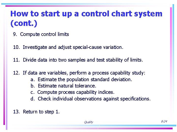
How to start up a control chart system (cont. ) 9. Compute control limits 10. Investigate and adjust special-cause variation. 11. Divide data into two samples and test stability of limits. 12. If data are variables, perform a process capability study: a. Estimate the population standard deviation. b. Estimate natural tolerance. c. Compute process capability indices. d. Check individual observations against specifications. 13. Return to step 1. Quality 8 -24

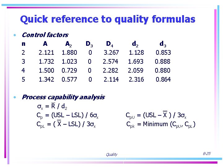
Quick reference to quality formulas • Control factors n A A 2 2 2. 121 1. 880 3 1. 732 1. 023 4 1. 500 0. 729 5 1. 342 0. 577 D 3 0 0 D 4 3. 267 2. 574 2. 282 2. 114 • Process capability analysis σx = R / d 2 Cp = (USL – LSL) / 6σx Cp. L = ( X – LSL) / 3σx d 2 1. 128 1. 693 2. 059 2. 316 d 3 0. 853 0. 888 0. 880 0. 864 Cp. U = (USL – X ) / 3σx Cpk = Minimum (Cp. U, Cp. L) Quality 8 -25

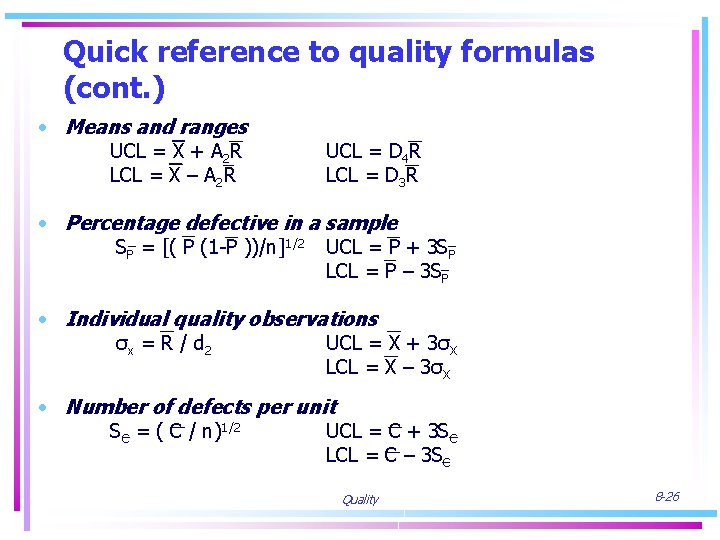
Quick reference to quality formulas (cont. ) • Means and ranges UCL = X + A 2 R LCL = X – A 2 R UCL = D 4 R LCL = D 3 R • Percentage defective in a sample SP = [( P (1 -P ))/n]1/2 UCL = P + 3 SP LCL = P – 3 SP • Individual quality observations σx = R / d 2 UCL = X + 3σX LCL = X – 3σX • Number of defects per unit SC = ( C / n)1/2 UCL = C + 3 SC LCL = C – 3 SC Quality 8 -26