Forecasting for Operations Everette S Gardner Jr Ph

Forecasting for Operations Everette S. Gardner, Jr. , Ph. D. Bauer College of Business University of Houston October 30, 2006

Forecasting for Operations • Operational systems typically include large numbers of time series. Problems in evaluating forecast accuracy: – – – – Pooled data structures Pooled averages Choice of error statistic Cumulating over lead times Stability of error measures across origins Method selection Product hierarchies • References – Tashman (IJF, 2000) – Fildes (Management Science, 1989; IJF, 1992) 2

Forecasting for Operations • We can bypass many of these problems by judging the impact of forecasting in financial or operational terms: – – – Customer service Inventory investment Purchasing workload Capacity requirements Production scheduling efficiency 3

Forecasting for Operations Case Studies: • Customer service – U. S. Navy distribution system • Inventory investment – Manufacturer of snack foods • Purchasing workload – Manufacturer/distributor of water filtration systems • Capacity requirements – Distributor of cleaning supplies • Production scheduling efficiency – Manufacturer of cookware 4

U. S. Navy distribution system • Scope – 50, 000 line items stocked at 11 supply centers – 240, 000 demand series – $425 million inventory investment • Decision Rules – Simple exponential smoothing – Replenishment by economic order quantity – Safety stocks set to minimize backorder delay 5

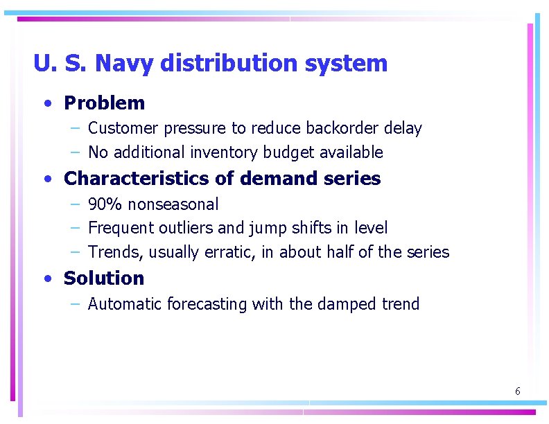
U. S. Navy distribution system • Problem – Customer pressure to reduce backorder delay – No additional inventory budget available • Characteristics of demand series – 90% nonseasonal – Frequent outliers and jump shifts in level – Trends, usually erratic, in about half of the series • Solution – Automatic forecasting with the damped trend 6

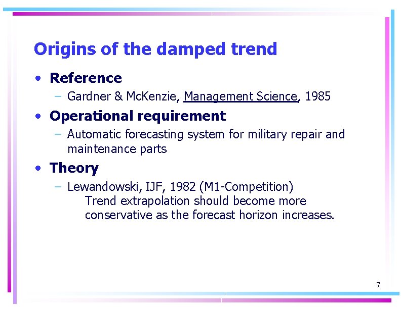
Origins of the damped trend • Reference – Gardner & Mc. Kenzie, Management Science, 1985 • Operational requirement – Automatic forecasting system for military repair and maintenance parts • Theory – Lewandowski, IJF, 1982 (M 1 -Competition) Trend extrapolation should become more conservative as the forecast horizon increases. 7

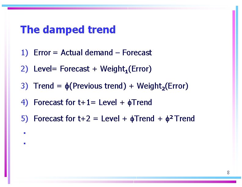
The damped trend 1) Error = Actual demand – Forecast 2) Level= Forecast + Weight 1(Error) 3) Trend = (Previous trend) + Weight 2(Error) 4) Forecast for t+1= Level + Trend 5) Forecast for t+2 = Level + Trend + 2 Trend. . 8

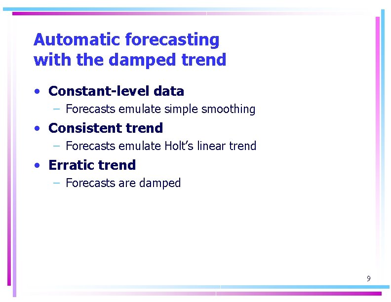
Automatic forecasting with the damped trend • Constant-level data – Forecasts emulate simple smoothing • Consistent trend – Forecasts emulate Holt’s linear trend • Erratic trend – Forecasts are damped 9

Automatic forecasting with the damped trend In constant-level data, the forecasts emulate simple exponential smoothing: 10

Automatic forecasting with the damped trend In data with a consistent trend and little noise, the forecasts emulate Holt’s linear trend: 11

Automatic forecasting with the damped trend When the trend is erratic, the forecasts are damped: 12

Automatic forecasting with the damped trend The damping effect increases with the level of noise in the data: 13

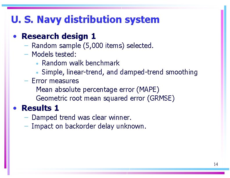
U. S. Navy distribution system • Research design 1 – Random sample (5, 000 items) selected. – Models tested: • Random walk benchmark • Simple, linear-trend, and damped-trend smoothing – Error measures Mean absolute percentage error (MAPE) Geometric root mean squared error (GRMSE) • Results 1 – Damped trend was clear winner. – Impact on backorder delay unknown. 14

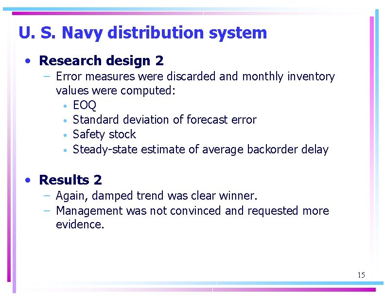
U. S. Navy distribution system • Research design 2 – Error measures were discarded and monthly inventory values were computed: • EOQ • Standard deviation of forecast error • Safety stock • Steady-state estimate of average backorder delay • Results 2 – Again, damped trend was clear winner. – Management was not convinced and requested more evidence. 15

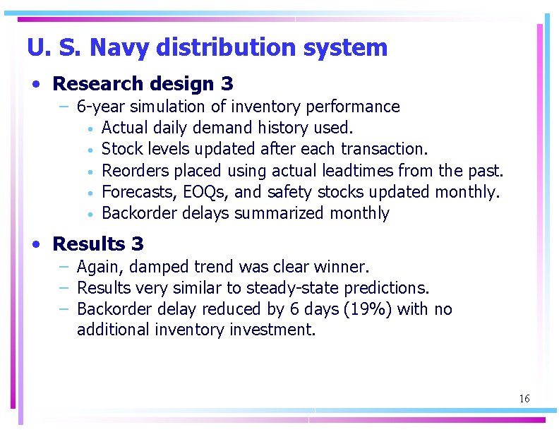
U. S. Navy distribution system • Research design 3 – 6 -year simulation of inventory performance • Actual daily demand history used. • Stock levels updated after each transaction. • Reorders placed using actual leadtimes from the past. • Forecasts, EOQs, and safety stocks updated monthly. • Backorder delays summarized monthly • Results 3 – Again, damped trend was clear winner. – Results very similar to steady-state predictions. – Backorder delay reduced by 6 days (19%) with no additional inventory investment. 16

Average delay in filling backorders U. S. Navy distribution system 17

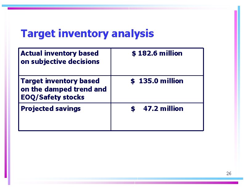
Snack-food manufacturer • Company – – Manufacturer of 80 snack foods Food inventories managed by commodity trading rules No formal decision rules for packaging inventories Subjective forecasting • Problem – Excess stocks of packaging materials – Difficult to set a target value for inventory investment on the balance sheet 18

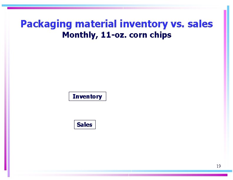
Packaging material inventory vs. sales Monthly, 11 -oz. corn chips Inventory Sales 19

Snack-food manufacturer Solution – Automatic forecasting with the damped trend – Replenishment by economic order quantity – Safety stocks set to meet target probability of shortage 20

Damped-trend performance 11 -oz. corn chips 21

Investment analysis 11 -oz. Corn chips 22

Safety stocks vs. shortages 11 -oz. Corn chips 23

Safety stocks vs. forecast errors 11 -oz. Corn chips Safety stock Forecast errors 24

Target inventory vs. sales Monthly, 11 -oz. corn chips Actual Inventory Target inventory Sales 25

Target inventory analysis Actual inventory based on subjective decisions $ 182. 6 million Target inventory based on the damped trend and EOQ/Safety stocks $ 135. 0 million Projected savings $ 47. 2 million 26

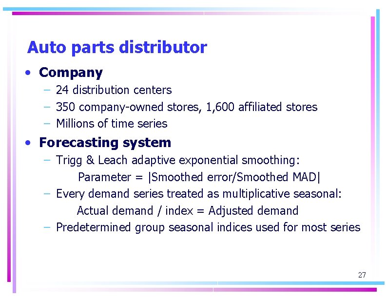
Auto parts distributor • Company – 24 distribution centers – 350 company-owned stores, 1, 600 affiliated stores – Millions of time series • Forecasting system – Trigg & Leach adaptive exponential smoothing: Parameter = |Smoothed error/Smoothed MAD| – Every demand series treated as multiplicative seasonal: Actual demand / index = Adjusted demand – Predetermined group seasonal indices used for most series 27

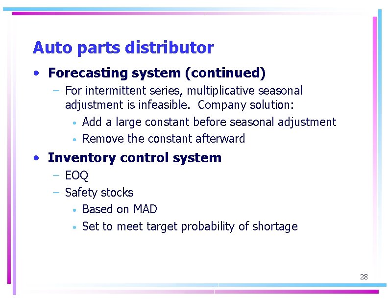
Auto parts distributor • Forecasting system (continued) – For intermittent series, multiplicative seasonal adjustment is infeasible. Company solution: • Add a large constant before seasonal adjustment • Remove the constant afterward • Inventory control system – EOQ – Safety stocks • Based on MAD • Set to meet target probability of shortage 28

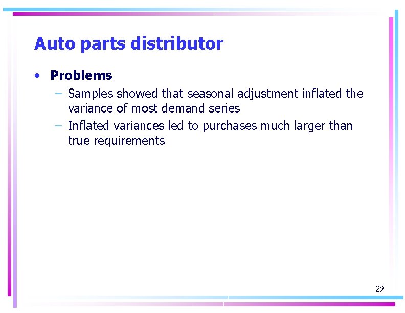
Auto parts distributor • Problems – Samples showed that seasonal adjustment inflated the variance of most demand series – Inflated variances led to purchases much larger than true requirements 29

Auto parts distributor: Example of inflated variance 30

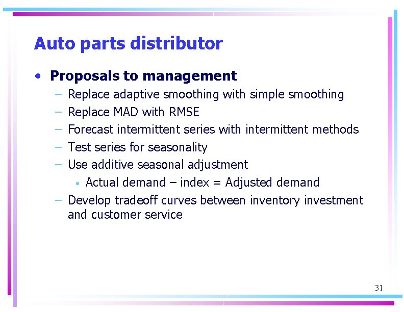
Auto parts distributor • Proposals to management – – – Replace adaptive smoothing with simple smoothing Replace MAD with RMSE Forecast intermittent series with intermittent methods Test series for seasonality Use additive seasonal adjustment • Actual demand – index = Adjusted demand – Develop tradeoff curves between inventory investment and customer service 31

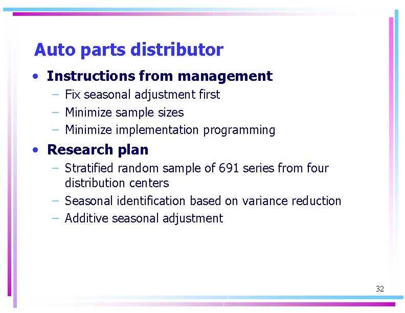
Auto parts distributor • Instructions from management – Fix seasonal adjustment first – Minimize sample sizes – Minimize implementation programming • Research plan – Stratified random sample of 691 series from four distribution centers – Seasonal identification based on variance reduction – Additive seasonal adjustment 32

Auto parts distributor Seasonal adjustment of continuous data 33

Auto parts distributor Seasonal adjustment of intermittent data 34

Auto parts distributor: Estimated savings 35

Auto parts distributor • Sensitivity analysis – Simple smoothing produced significantly smaller safety stocks than adaptive smoothing – Periodic refitting of the simple smoothing model did not improve results – Replacement of the MAD with the RMSE made little difference in safety stocks – Autocorrelation analysis was no better than the simple variance test for seasonal identification – Croston’s method for intermittent data was no better than simple smoothing 36

Auto parts distributor • Lessons – It is dangerous to ignore seasonality testing in inventory series – It is dangerous to assume that every seasonal time series is multiplicative – Group seasonal indices can perform poorly in noisy data 37

Cookware manufacturer Number of production set-ups per month (Exponential smoothing implemented in May) 38

Cookware manufacturer Production runs by color, before and after exponential smoothing 39

Conclusions • Judge forecast accuracy in financial or operational terms – – Customer service Inventory investment on the balance sheet Purchasing workload Capacity requirements • Benchmark forecast accuracy with exponential smoothing 40