Efficient Algorithms for Nonparametric Clustering With Clutter WengKeen

Efficient Algorithms for Non-parametric Clustering With Clutter Weng-Keen Wong Andrew Moore (In partial fulfillment of the speaking requirement) 1

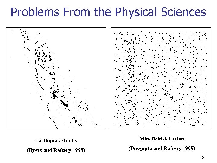
Problems From the Physical Sciences Earthquake faults Minefield detection (Byers and Raftery 1998) (Dasgupta and Raftery 1998) 2

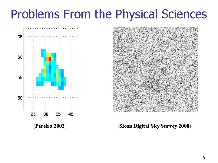
Problems From the Physical Sciences (Pereira 2002) (Sloan Digital Sky Survey 2000) 3

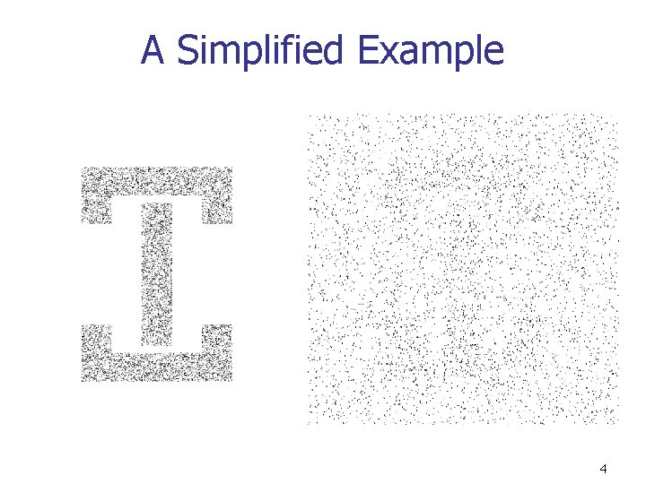
A Simplified Example 4

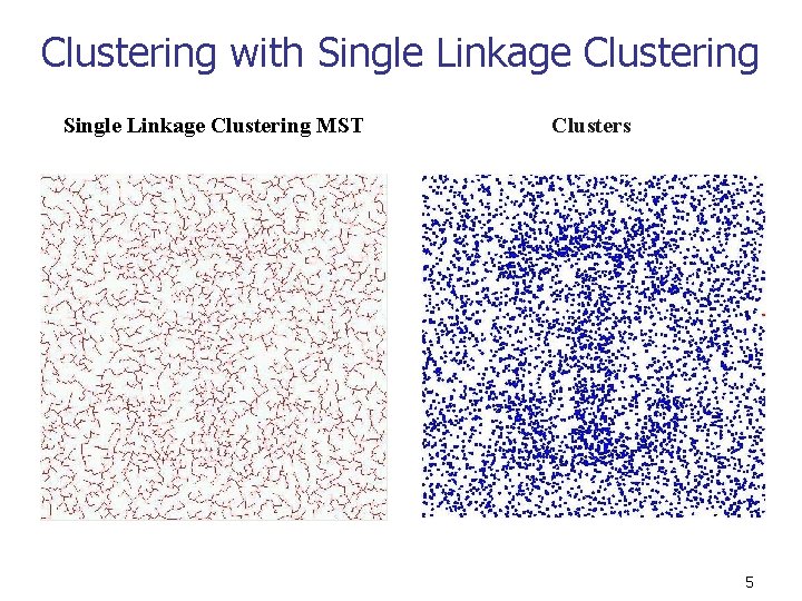
Clustering with Single Linkage Clustering MST Clusters 5

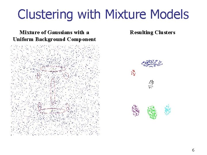
Clustering with Mixture Models Mixture of Gaussians with a Uniform Background Component Resulting Clusters 6

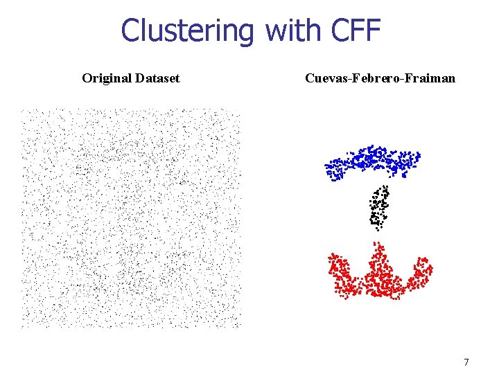
Clustering with CFF Original Dataset Cuevas-Febrero-Fraiman 7

Related Work (Dasgupta and Raftery 98) n Mixture model approach – mixture of Gaussians for features, Poisson process for clutter (Byers and Raftery 98) n K-nearest neighbour distances for all points modeled as a mixture of two gamma distributions, one for clutter and one for the features n Classify each data point based on which component it was most likely generated from 8

Outline 1. Introduction: Clustering and Clutter 2. The Cuevas-Febreiro-Fraiman Algorithm 3. Optimizing Step One of CFF 4. Optimizing Step Two of CFF 5. Results 9

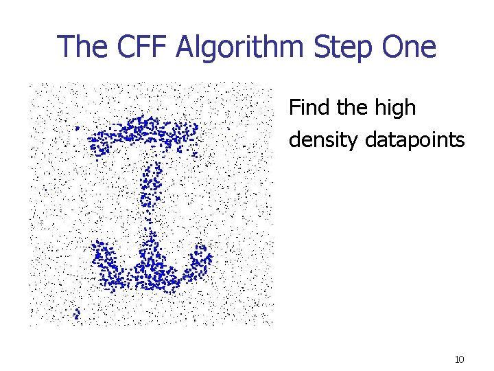
The CFF Algorithm Step One Find the high density datapoints 10

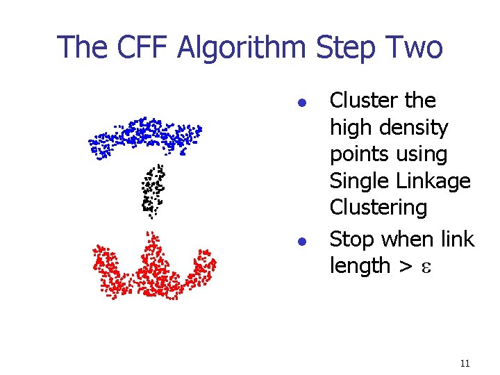
The CFF Algorithm Step Two l l Cluster the high density points using Single Linkage Clustering Stop when link length > 11

The CFF Algorithm n n Originally intended to estimate the number of clusters Can also be used to find clusters against a noisy background 12

Step One: Density Estimators n n n Finding high density points requires a density estimator Want to make as few assumptions about underlying density as possible Use a non-parametric density estimator 13

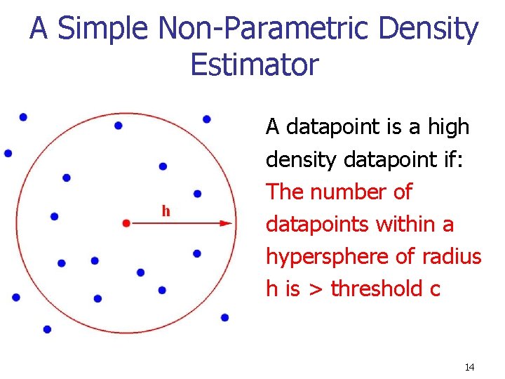
A Simple Non-Parametric Density Estimator A datapoint is a high density datapoint if: The number of datapoints within a hypersphere of radius h is > threshold c 14

Speeding up the Non-Parametric Density Estimator n n Addressed in a separate paper (Gray and Moore 2001) Two basic ideas: 1. Use a dual tree algorithm (Gray and Moore 2000) 2. Cut search off early without computing exact densities (Moore 2000) 15

Step Two: Euclidean Minimum Spanning Trees (EMSTs) n n n Traditional MST algorithms assume you are given all the distances Implies O(N 2) memory usage Want to use a Euclidean Minimum Spanning Tree algorithm 16

Optimizing Clustering Step n n Exploit recent results in computational geometry for efficient EMSTs Involves modification to Geo. MST 2 algorithm by (Narasimhan et al 2000) Geo. MST 2 is based on Well-Separated Pairwise Decompositions (WSPDs) (Callahan 1995) Our optimizations gain an order of magnitude speedup, especially in higher dimensions 17

Outline for Optimizing Step Two 1. 2. 3. 4. 5. High level overview of Geo. MST 2 Properties of a WSPD How to create a WSPD More detailed description of Geo. MST 2 Our optimizations 18

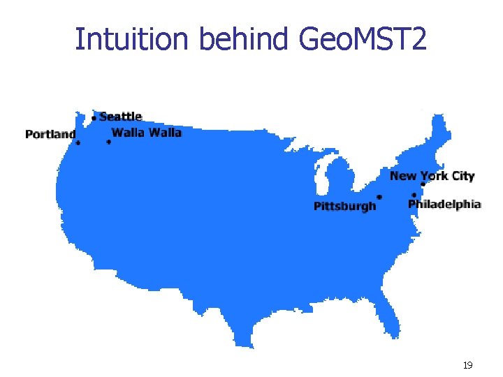
Intuition behind Geo. MST 2 19

Intuition behind Geo. MST 2 20

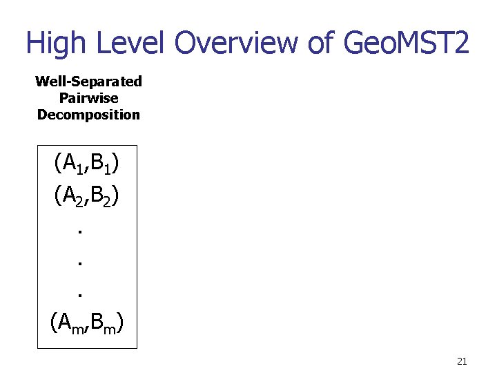
High Level Overview of Geo. MST 2 Well-Separated Pairwise Decomposition (A 1, B 1) (A 2, B 2). . . (Am, Bm) 21

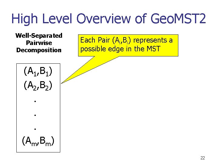
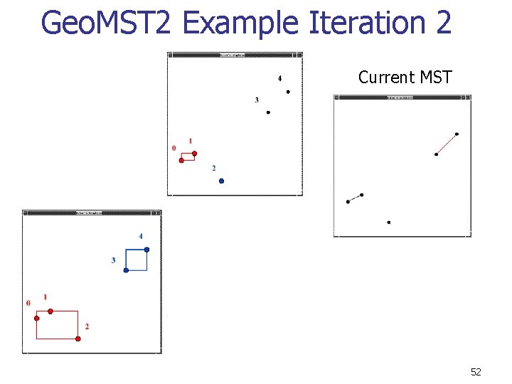
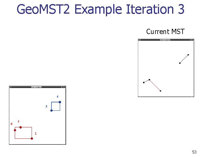
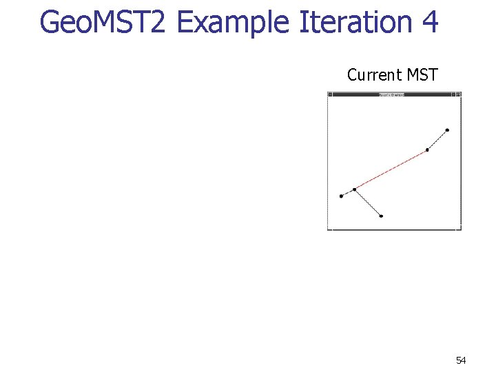
High Level Overview of Geo. MST 2 Well-Separated Pairwise Decomposition Each Pair (Ai, Bi) represents a possible edge in the MST (A 1, B 1) (A 2, B 2). . . (Am, Bm) 22

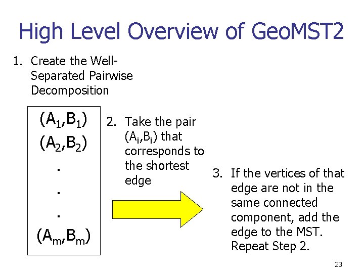
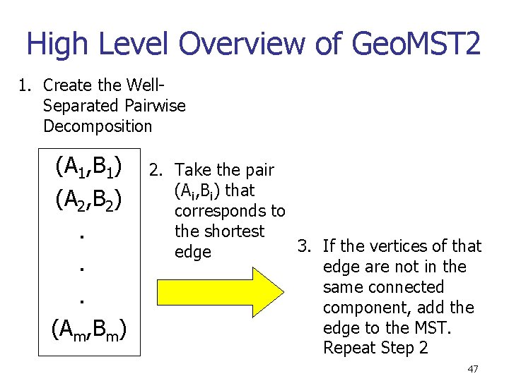
High Level Overview of Geo. MST 2 1. Create the Well. Separated Pairwise Decomposition (A 1, B 1) (A 2, B 2). . . (Am, Bm) 2. Take the pair (Ai, Bi) that corresponds to the shortest 3. If the vertices of that edge are not in the same connected component, add the edge to the MST. Repeat Step 2. 23

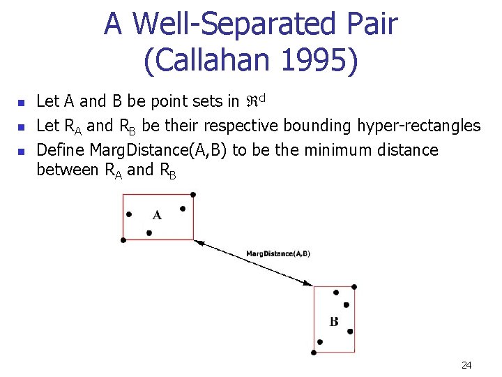
A Well-Separated Pair (Callahan 1995) n n n Let A and B be point sets in d Let RA and RB be their respective bounding hyper-rectangles Define Marg. Distance(A, B) to be the minimum distance between RA and RB 24

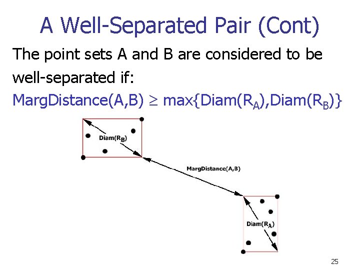
A Well-Separated Pair (Cont) The point sets A and B are considered to be well-separated if: Marg. Distance(A, B) max{Diam(RA), Diam(RB)} 25

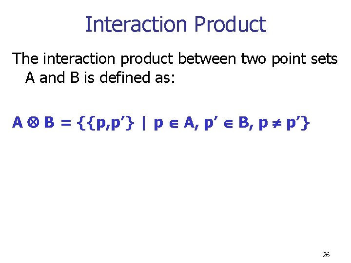
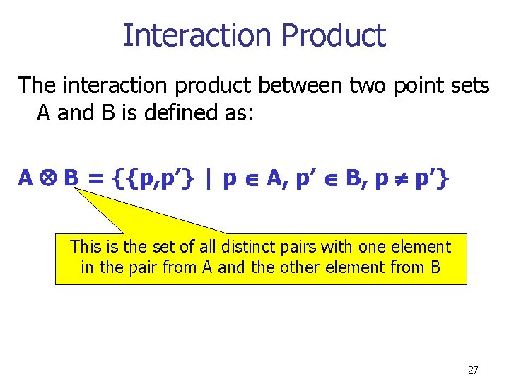
Interaction Product The interaction product between two point sets A and B is defined as: A B = {{p, p’} | p A, p’ B, p p’} 26

Interaction Product The interaction product between two point sets A and B is defined as: A B = {{p, p’} | p A, p’ B, p p’} This is the set of all distinct pairs with one element in the pair from A and the other element from B 27

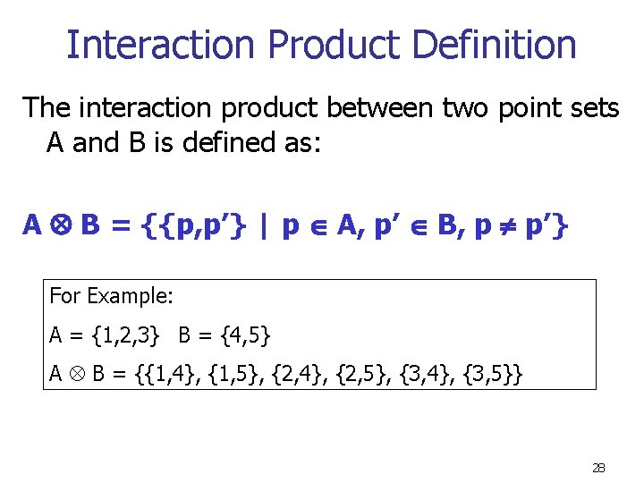
Interaction Product Definition The interaction product between two point sets A and B is defined as: A B = {{p, p’} | p A, p’ B, p p’} For Example: A = {1, 2, 3} B = {4, 5} A B = {{1, 4}, {1, 5}, {2, 4}, {2, 5}, {3, 4}, {3, 5}} 28

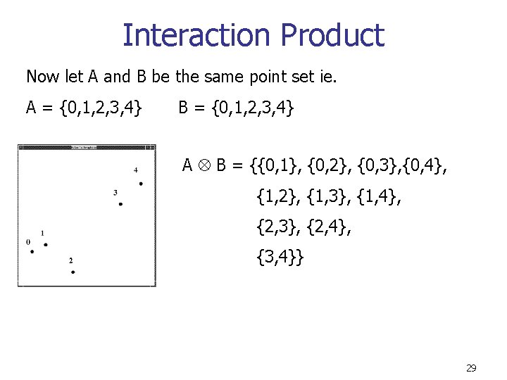
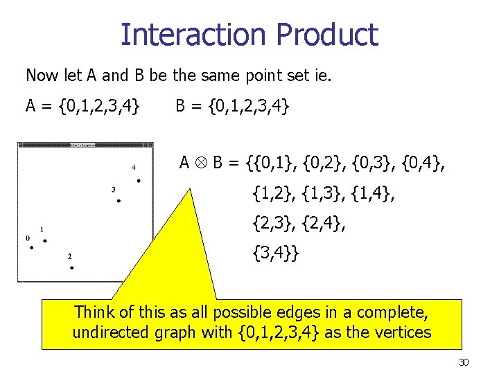
Interaction Product Now let A and B be the same point set ie. A = {0, 1, 2, 3, 4} B = {0, 1, 2, 3, 4} A B = {{0, 1}, {0, 2}, {0, 3}, {0, 4}, {1, 2}, {1, 3}, {1, 4}, {2, 3}, {2, 4}, {3, 4}} 29

Interaction Product Now let A and B be the same point set ie. A = {0, 1, 2, 3, 4} B = {0, 1, 2, 3, 4} A B = {{0, 1}, {0, 2}, {0, 3}, {0, 4}, {1, 2}, {1, 3}, {1, 4}, {2, 3}, {2, 4}, {3, 4}} Think of this as all possible edges in a complete, undirected graph with {0, 1, 2, 3, 4} as the vertices 30

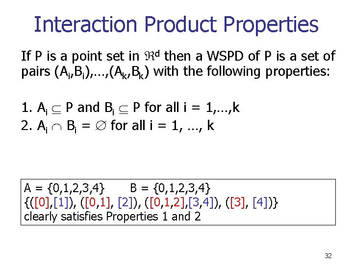
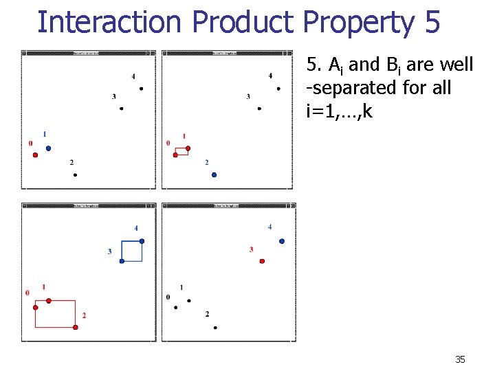
A Well-Separated Pairwise Decomposition Pair #1: Pair #2: Pair #3: Pair #4: ([0], [1]) ([0, 1], [2]) ([0, 1, 2], [3, 4]) ([3], [4]) Claim: The set of pairs {([0], [1]), ([0, 1], [2]), ([0, 1, 2], [3, 4]), ([3], [4])} form a Well-Separated Decomposition. 31

Interaction Product Properties If P is a point set in d then a WSPD of P is a set of pairs (Ai, Bi), …, (Ak, Bk) with the following properties: 1. Ai P and Bi P for all i = 1, …, k 2. Ai Bi = for all i = 1, …, k A = {0, 1, 2, 3, 4} B = {0, 1, 2, 3, 4} {([0], [1]), ([0, 1], [2]), ([0, 1, 2], [3, 4]), ([3], [4])} clearly satisfies Properties 1 and 2 32

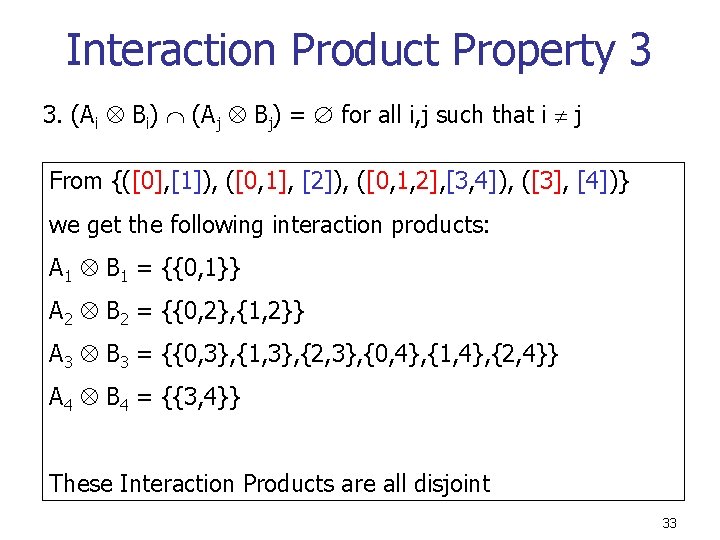
Interaction Product Property 3 3. (Ai Bi) (Aj Bj) = for all i, j such that i j From {([0], [1]), ([0, 1], [2]), ([0, 1, 2], [3, 4]), ([3], [4])} we get the following interaction products: A 1 B 1 = {{0, 1}} A 2 B 2 = {{0, 2}, {1, 2}} A 3 B 3 = {{0, 3}, {1, 3}, {2, 3}, {0, 4}, {1, 4}, {2, 4}} A 4 B 4 = {{3, 4}} These Interaction Products are all disjoint 33

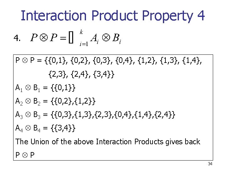
Interaction Product Property 4 4. P P = {{0, 1}, {0, 2}, {0, 3}, {0, 4}, {1, 2}, {1, 3}, {1, 4}, {2, 3}, {2, 4}, {3, 4}} A 1 B 1 = {{0, 1}} A 2 B 2 = {{0, 2}, {1, 2}} A 3 B 3 = {{0, 3}, {1, 3}, {2, 3}, {0, 4}, {1, 4}, {2, 4}} A 4 B 4 = {{3, 4}} The Union of the above Interaction Products gives back P P 34

Interaction Product Property 5 5. Ai and Bi are well -separated for all i=1, …, k 35

Two Points to Note about WSPDs n n Two distinct points are considered to be well-separated For any data set of size n, there is a trivial WSPD of size (n choose 2) 36

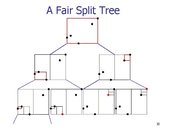
A Well-Separated Pairwise Decomposition (Continued) If there are n points in P, a WSPD of P can be constructed in O(nlogn) time with O(n) elements using a fair split tree (Callahan 1995) 37

A Fair Split Tree 38

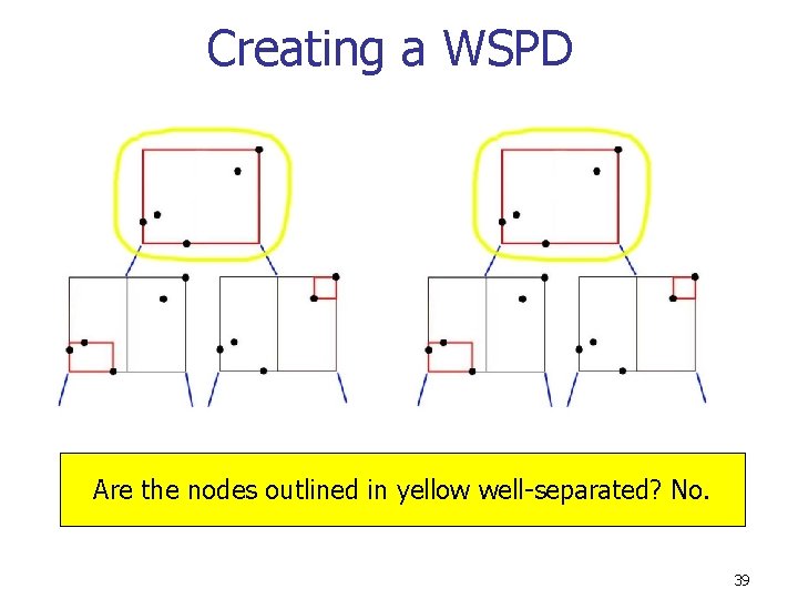
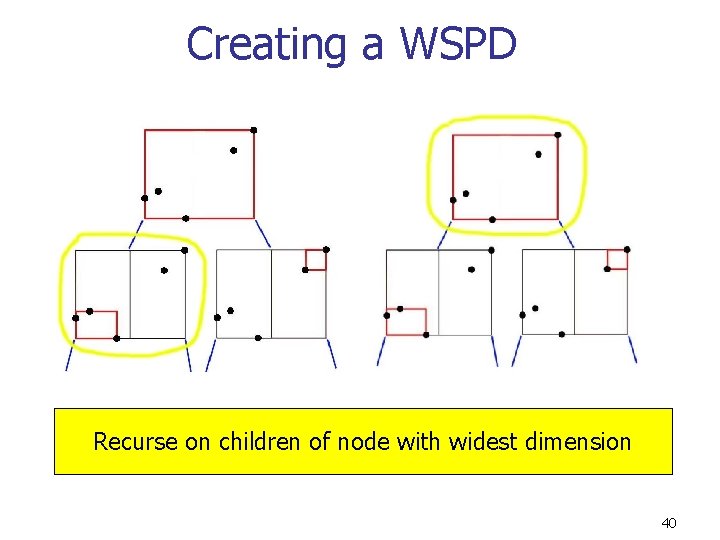
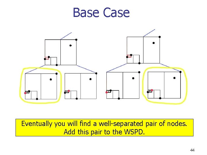
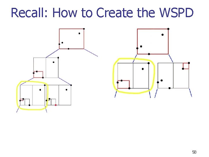
Creating a WSPD Are the nodes outlined in yellow well-separated? No. 39

Creating a WSPD Recurse on children of node with widest dimension 40

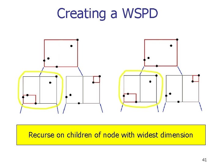
Creating a WSPD Recurse on children of node with widest dimension 41

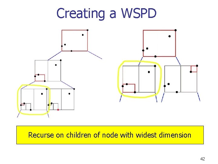
Creating a WSPD Recurse on children of node with widest dimension 42

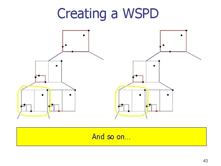
Creating a WSPD And so on… 43

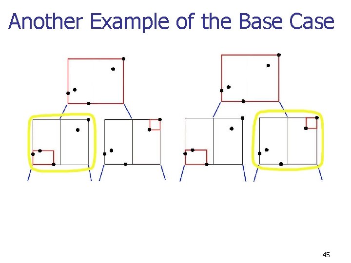
Base Case Eventually you will find a well-separated pair of nodes. Add this pair to the WSPD. 44

Another Example of the Base Case 45

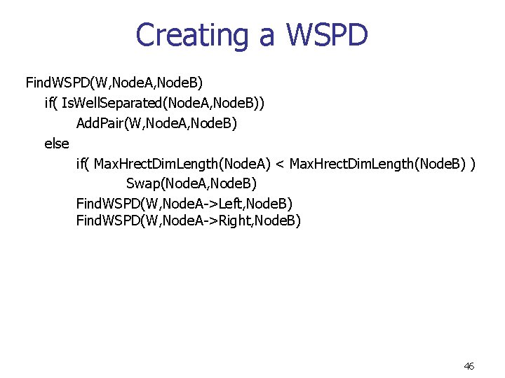
Creating a WSPD Find. WSPD(W, Node. A, Node. B) if( Is. Well. Separated(Node. A, Node. B)) Add. Pair(W, Node. A, Node. B) else if( Max. Hrect. Dim. Length(Node. A) < Max. Hrect. Dim. Length(Node. B) ) Swap(Node. A, Node. B) Find. WSPD(W, Node. A->Left, Node. B) Find. WSPD(W, Node. A->Right, Node. B) 46

High Level Overview of Geo. MST 2 1. Create the Well. Separated Pairwise Decomposition (A 1, B 1) (A 2, B 2). . . (Am, Bm) 2. Take the pair (Ai, Bi) that corresponds to the shortest 3. If the vertices of that edge are not in the same connected component, add the edge to the MST. Repeat Step 2 47

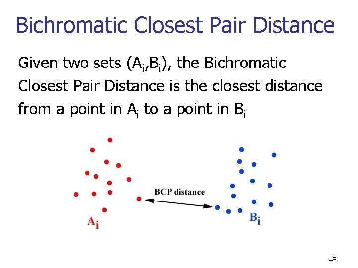
Bichromatic Closest Pair Distance Given two sets (Ai, Bi), the Bichromatic Closest Pair Distance is the closest distance from a point in Ai to a point in Bi 48

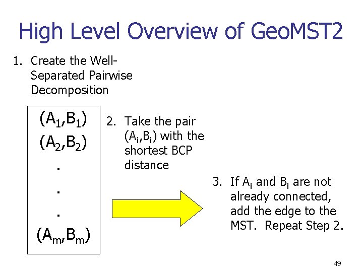
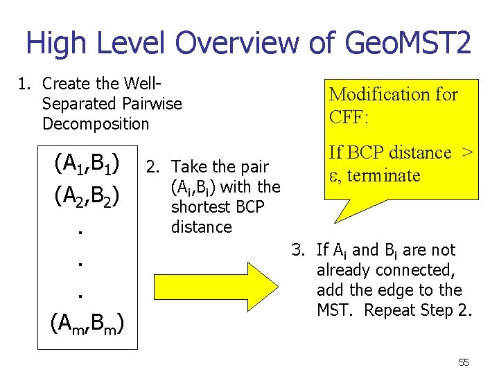
High Level Overview of Geo. MST 2 1. Create the Well. Separated Pairwise Decomposition (A 1, B 1) (A 2, B 2). . . (Am, Bm) 2. Take the pair (Ai, Bi) with the shortest BCP distance 3. If Ai and Bi are not already connected, add the edge to the MST. Repeat Step 2. 49

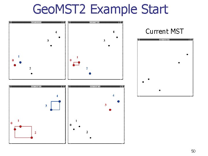
Geo. MST 2 Example Start Current MST 50

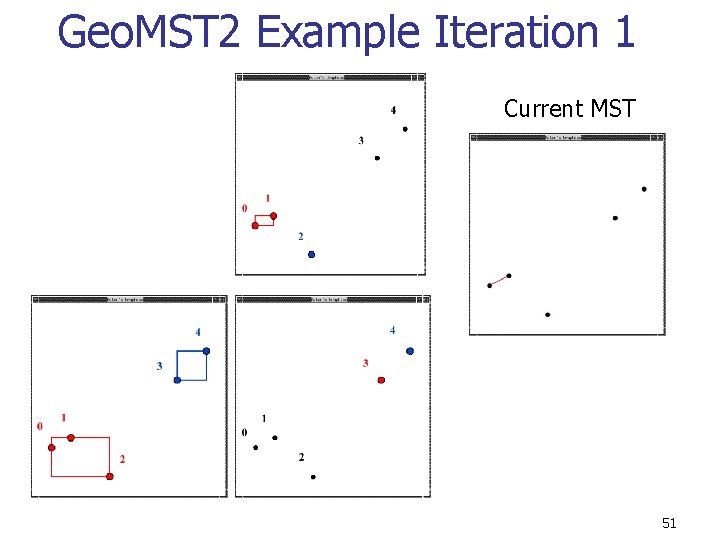
Geo. MST 2 Example Iteration 1 Current MST 51

Geo. MST 2 Example Iteration 2 Current MST 52

Geo. MST 2 Example Iteration 3 Current MST 53

Geo. MST 2 Example Iteration 4 Current MST 54

High Level Overview of Geo. MST 2 1. Create the Well. Separated Pairwise Decomposition (A 1, B 1) (A 2, B 2). . . (Am, Bm) 2. Take the pair (Ai, Bi) with the shortest BCP distance Modification for CFF: If BCP distance > , terminate 3. If Ai and Bi are not already connected, add the edge to the MST. Repeat Step 2. 55

Optimizations n n n We don’t need the EMST We just need to cluster all points that are within distance or less from each other Allows two optimizations to Geo. MST 2 code 56

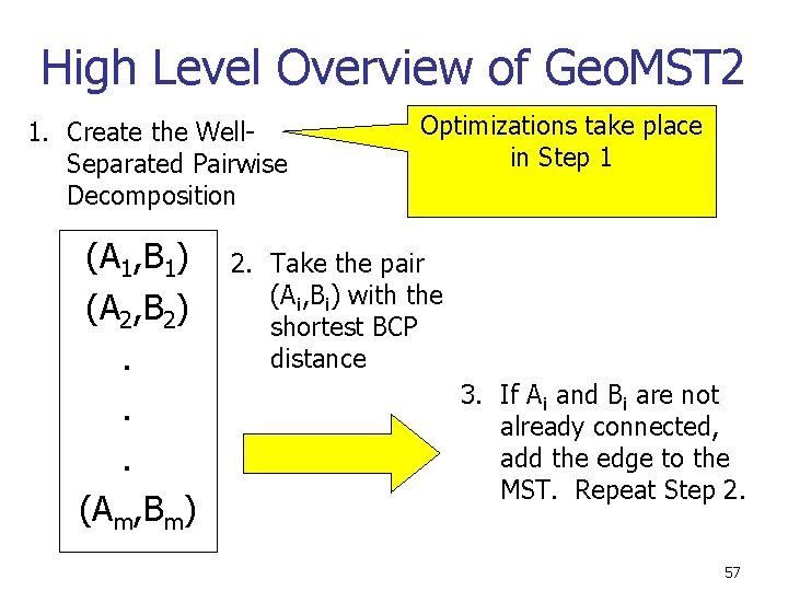
High Level Overview of Geo. MST 2 1. Create the Well. Separated Pairwise Decomposition (A 1, B 1) (A 2, B 2). . . (Am, Bm) Optimizations take place in Step 1 2. Take the pair (Ai, Bi) with the shortest BCP distance 3. If Ai and Bi are not already connected, add the edge to the MST. Repeat Step 2. 57

Recall: How to Create the WSPD 58

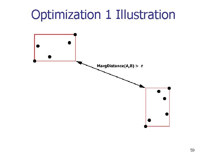
Optimization 1 Illustration 59

Optimization 1 Ignore all links that are > n Every pair (Ai, Bi) in the WSPD becomes an edge unless it joins two already connected components n If Marg. Distance(Ai, Bi) > , then an edge of length cannot exist between a point in Ai and Bi n Don’t include such a pair in the WSPD 60

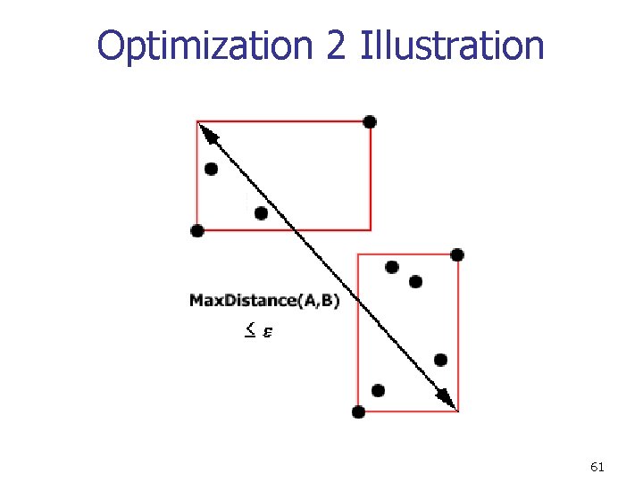
Optimization 2 Illustration 61

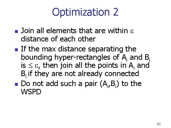
Optimization 2 n n n Join all elements that are within distance of each other If the max distance separating the bounding hyper-rectangles of Ai and Bi is , then join all the points in Ai and Bi if they are not already connected Do not add such a pair (Ai, Bi) to the WSPD 62

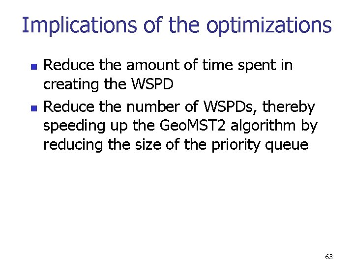
Implications of the optimizations n n Reduce the amount of time spent in creating the WSPD Reduce the number of WSPDs, thereby speeding up the Geo. MST 2 algorithm by reducing the size of the priority queue 63

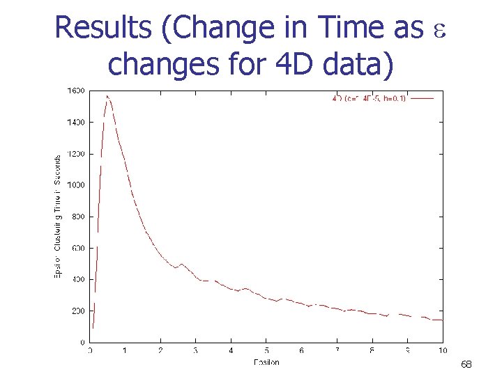
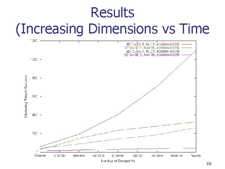
Results n n n Ran step two algorithms on subsets of the Sloan Digital Sky Survey 7 attributes – 4 colors, 2 sky coordinates, 1 redshift value Compared Kruskal, Geo. MST 2, and -clustering 64

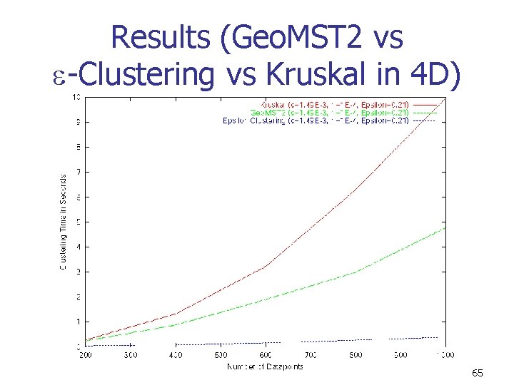
Results (Geo. MST 2 vs -Clustering vs Kruskal in 4 D) 65

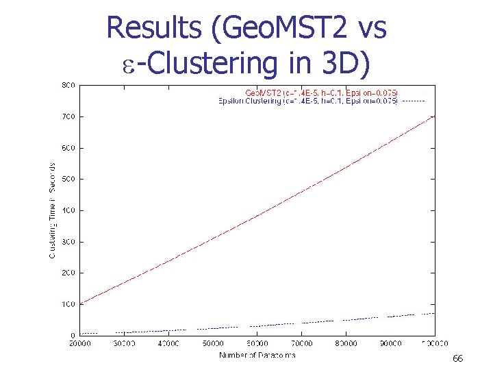
Results (Geo. MST 2 vs -Clustering in 3 D) 66

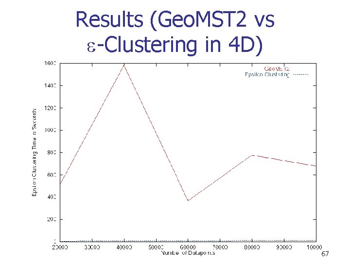
Results (Geo. MST 2 vs -Clustering in 4 D) 67

Results (Change in Time as changes for 4 D data) 68

Results (Increasing Dimensions vs Time 69

Future Work n n n More accurate, faster non-parametric density estimator Use ball trees instead of fair split tree Optimize algorithm if we keep h constant but vary c and 70

Conclusions n n -clustering outperforms Geo. MST 2 by nearly an order of magnitude in higher dimensions Combining the optimizations in both steps will yield an efficient algorithm for clustering against clutter on massive data sets 71