Lecture 12 Clustering What is Clustering Clustering is

Lecture 12 Clustering

What is Clustering? • Clustering is an EXPLORATORY statistical technique used to break up a data set into smaller groups or “clusters” with the idea that objects within a cluster are similar and objects in different clusters are different. • It uses different distance measures between units of a group and across groups to decide which units fall in a group.

Clustering: some thoughts • Biologists really LOVE clustering, and believe that clustering can produce “discoveries” of patterns. • Statisticians for the most part are somewhat skeptical about these methods. • Clustering is called “unsupervised learning” by computer scientists and “class discovery” by micro-array biologists. • Though clustering DOES provide clusters or smaller groups, keep in mind that to interpret them you need to know the epidemiological and technical aspect of the study.

Keep in mind • Epidemiological aspects of the study: experiment or observational study, and if the latter, knowledge of possible confounders; relation between training and test sets; relation between current data and future data to which results might be applied, … • Technical aspects of the study: tissue collection, storage and processing procedures, microarray assays and analyses, focussing on the role of time, place, personnel, reagents, and methods used, including evidence of design, randomization, blinding, to avoid or correct for possible confounding…. • In other contexts, and possibly in these, the results have been driven by study inadequacies rather than by biology. Beware!

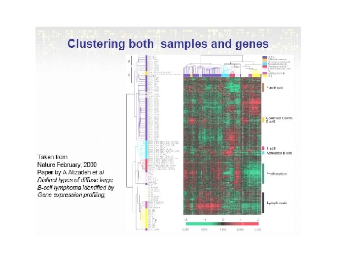
Clustering in MA • Idea: to group observations that are “similar” based on predefined criteria. • Clustering can be applied to rows (genes) and/or columns (arrays) of an expression data matrix. • Clustering allows for reordering of the rows/columns of an expression data matrix which is appropriate for visualization. • Fundamentally an exploratory tool, clustering is firmly imbedded in many biologists’ minds as the statistical method for the analysis of microarray gene expression data. Worrying, but an opportunity!

Aim and End product of clustering • • Clustering leads to readily interpretable figures and can be helpful for identifying patterns in time or space, especially artifacts! Examples: We can cluster cell samples (columns), e. g. 1) for identification (profiles). Here, we might want to estimate the number of different neuronal cell types in a set of samples, based on gene expression measurements. 2) the identification of new / unknown tumor classes using gene expression profiles. • We can cluster genes (rows) , e. g. 1) using large numbers of yeast experiments, to identify groups of co-regulated genes. These are usually interpreted and subjected to further analysis. 2) to reduce redundancy (cf. variable selection) in predictive models. • BIOLOGIST like the latter, but it is often NOT practical to do.

Why Cluster Samples? • There are very few formal theories about clustering though intuitively the idea is: • cluster the internal cohesion and external isolation. • Time-course experiments are often clustered to see if there are developmental similarities. • Useful for visualization. • Generally considered appropriate in typical clinical experiments.

Clustering • How is “closeness decided”? • For clustering we generally need two ideas: • Distance: the original distance used to measure the distance between two points • Linkage: condensation of each group of observations into a single representative point

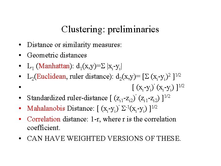
Clustering: preliminaries • • Distance or similarity measures: Geometric distances L 1 (Manhattan): d 1(x, y)=S |xi-yi| L 2(Euclidean, ruler distance): d 2(x, y)= [S (xi-yi)2 ]1/2 [ (xi-yi)’ (xi-yi) ]1/2 Standardized ruler-distance [ (zi 1 -zi 2)’ (zi 1 -zi 2) ]1/2 Mahalanobis Distance: [ (xi-yi)’ S-1(xi-yi) ]1/2 Correlation distance: 1 -r, where r is the correlation coefficient. • CAN HAVE WEIGHTED VERSIONS OF THESE.

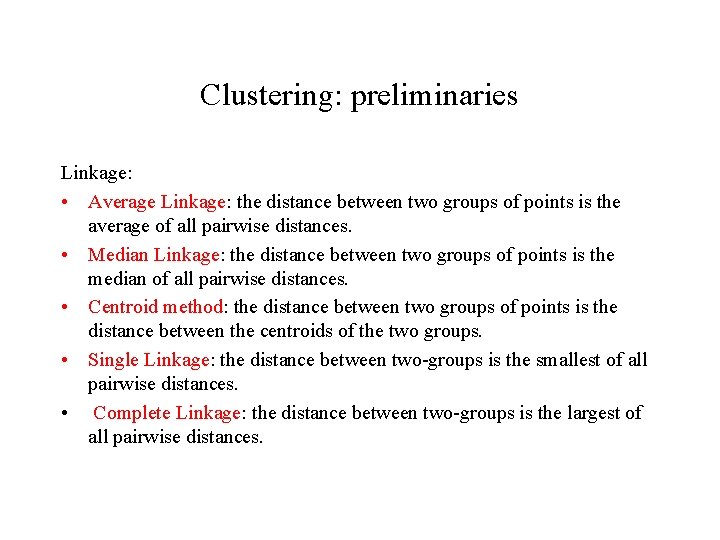
Clustering: preliminaries Linkage: • Average Linkage: the distance between two groups of points is the average of all pairwise distances. • Median Linkage: the distance between two groups of points is the median of all pairwise distances. • Centroid method: the distance between two groups of points is the distance between the centroids of the two groups. • Single Linkage: the distance between two-groups is the smallest of all pairwise distances. • Complete Linkage: the distance between two-groups is the largest of all pairwise distances.

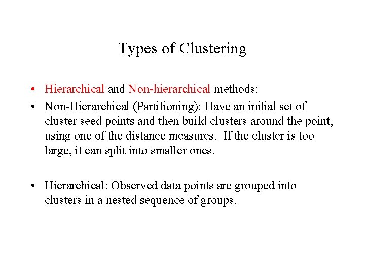
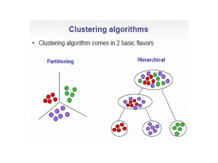
Types of Clustering • Hierarchical and Non-hierarchical methods: • Non-Hierarchical (Partitioning): Have an initial set of cluster seed points and then build clusters around the point, using one of the distance measures. If the cluster is too large, it can split into smaller ones. • Hierarchical: Observed data points are grouped into clusters in a nested sequence of groups.

Non-hierarchical: Partitioning methods Partition the data into a pre-specified number k of mutually exclusive and exhaustive groups. Iteratively reallocate the observations to clusters until some criterion is met, e. g. minimize within cluster sums of squares. Issues: Need to know the seeds and the number of clusters to start off with. If one uses the computer the pick the seeds the order of entry of the data may make a difference.

Hierarchical methods • Hierarchical clustering methods produce a tree or dendrogram often usingle-link clustering methods • They avoid specifying how many clusters are appropriate by providing a partition for each k obtained from cutting the tree at some level. • The tree can be built in two distinct ways - bottom-up: agglomerative clustering. ** - top-down: divisive clustering.

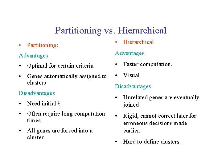
Partitioning vs. Hierarchical • Partitioning: • Hierarchical Advantages • Optimal for certain criteria. • Faster computation. • Genes automatically assigned to clusters • Visual. Disadvantages • Need initial k; • Often require long computation times. • All genes are forced into a cluster. Disadvantages • Unrelated genes are eventually joined • Rigid, cannot correct later for erroneous decisions made earlier. • Hard to define clusters.

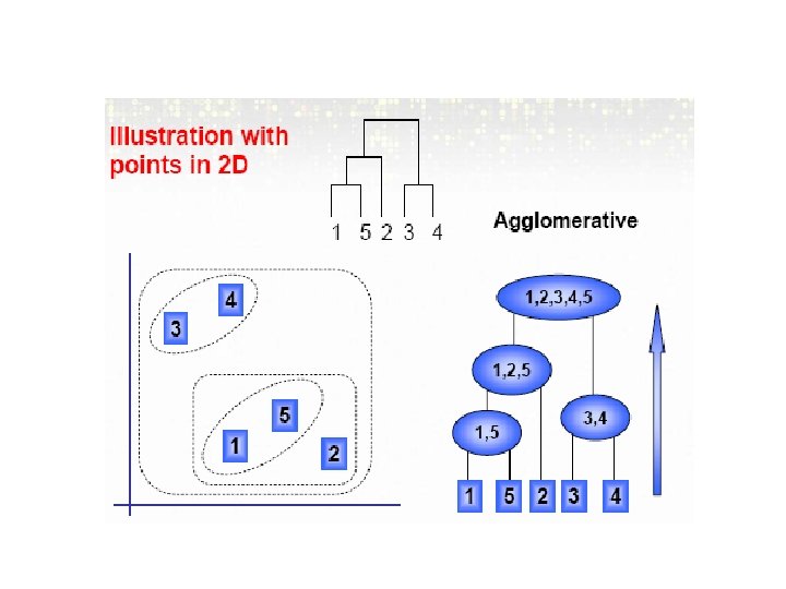
Bottom-up- Agglomerative Method • This is the most common used method and produces the famous tree-diagram. • VERY common in MA literature, first introduced by Eisen (1998). • Start with n m. RNA sample (or g gene) clusters • At each step, merge the two closest clusters using a measure of between-cluster dissimilarity which reflects the shape of the clusters • The distance between clusters is defined by the method used (e. g. , if complete linkage, the distance is defined as the distance between furthest pair of points in the two clusters)

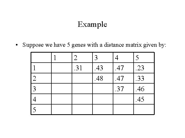
Example • Suppose we have 5 genes with a distance matrix given by: 1 1 2 3 4 5 2. 31 3. 48 4. 47. 37 5. 23. 33. 46. 45

Example • First we have 5 clusters: • C 0 = {[1], [2], [3], [4], [5]} • Since 1 and 5 have the least distance they are combined and C 1 = {[1, 5], [2], [3], [4]} • And C 2= {[1, 5], [2], [3, 4]} • And C 3= {[1, 5, 2], [3, 4]} • And C 4= {[1, 5, 2, 3, 4]}

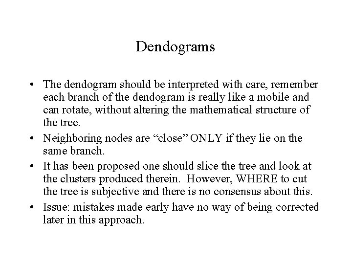
Dendograms • The dendogram should be interpreted with care, remember each branch of the dendogram is really like a mobile and can rotate, without altering the mathematical structure of the tree. • Neighboring nodes are “close” ONLY if they lie on the same branch. • It has been proposed one should slice the tree and look at the clusters produced therein. However, WHERE to cut the tree is subjective and there is no consensus about this. • Issue: mistakes made early have no way of being corrected later in this approach.

Two-way Clustering • Refers to methods that use samples and genes simultaneously to extract information. Some examples: • - Block Clustering (Hartigan, 1972) which repeatedly rearranges rows and columns to obtain the largest reduction of total within block variance. • - Plaid Models (Lazzeroni and Owen, 2002) • - Friedman and Meulmann (2002) present an algorithm to cluster samples based on the subsets of attributes, i. e. each group of samples could have been characterized by different gene sets.

How many clusters? A brief discussion • Global Criteria: 1. Statistics based on within- and between-clusters matrices of sumsofsquares and cross-products (30 methods reviewed by Milligan & Cooper, 1985). 2. Average silhouette (Kaufman & Rousseeuw, 1990). 3. Graph theory (e. g. : cliques in CAST) (Ben-Dor et al. , 1999). 4. Model-based methods: EM algorithm for Gaussian mixtures, Fraley & Raftery (1998, 2000) and Mc. Lachlan et al. (2001). • Resampling methods: 1. Gap statistic (Tibshirani et al. , 2000). 2. WADP (Bittner et al. , 2000). 3. Clest (Dudoit & Fridlyand, 2001). 4. Boostrap (van der Laan & Pollard, 2001).

Some remarks on clustering- 1 • Simplistically, clustering cannot fail. That is, every clustering method will return clusters, whether the data are organized in clusters or not. • Clustering helps to group / order information and is a visualization tool for learning about the data. However, clustering results do not provide any kind of “proof” of anything.

Some remarks-II • One of the more paradoxical aspects of clustering is that it gets used in biology, even when class labels are available instead of using a discrimination method. • The idea is: it is somehow seen as less “biased” to demonstrate the ability of the data to produce the class differences without using class labels. • When the inferred clusters largely coincide with the known classes, this is thought to “validate” the class labels. • The illogicality and inefficiency of this process does not seem to have become widely appreciated. One sees different “classifiers” (e. g. different gene sets) compared w. r. t their ability to separate known classes, simply by inspecting the clustering they produce, rather than by building classifiers.

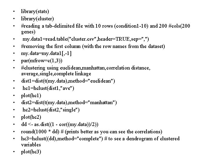
• • • • • library(stats) library(cluster) #reading a tab-delimited file with 10 rows (condition 1 -10) and 200 #cols(200 genes) my. data 1=read. table("cluster. csv", header=TRUE, sep=", ") #removing the first column (with the row names from the dataset) my. data=my. data 1[, -1] par(mfrow=c(1, 3)) #clustering using euclidean, manhattan, correlation distance, average, single, complete linkage dist 1=dist(t(my. data), method="euclidean") hc 1=hclust(dist 1, "ave") plot(hc 1) dist 2=dist(t(my. data), method="manhattan") hc 2=hclust(dist 2, "single") plot(hc 2) dd <- as. dist((1 - cor((my. data))/2)) round(1000 * dd) # (prints better as you can see the correlations) hc 3=hclust((dd), method="complete") # to see a dendrogram of clustered variables plot(hc 3)