CS 367 Introduction to Data Structures Lecture 22

CS 367 Introduction to Data Structures Lecture 22

Today’s topics: u Graphs u Depth-First Search u Graph Algorithms

Epic Picnic When: Tuesday, April 17 th, 5: 457: 30 pm Where: Epic Campus, Verona – Voyager Hall – MIR Commons Transportation: Shuttles will depart at approximately 5: 15 pm, 5: 30 pm and 5: 45 pm. Return shuttles will leave Epic at approximately 7: 00 pm, 7: 15 pm and 7: 30 pm. Dress: Casual

Graphs A generalization of trees • Graphs have nodes and edges (Sometimes called vertices and arcs) • Nodes can have any number of incoming edges. • Every tree is a graph, but not all graphs are trees •

Directed and Undirected Graphs Edges may have a direction (be an arrow) or may be undirected (just a line)

In a directed graph you must follow the direction of the arrow • In an undirected graph you may go in either direction • Directed graphs may reach a “dead end” •

Graph Terminology The two nodes are adjacent (they are neighbors). • Node 2 is a predecessor of node 1. • Node 1 is a successor of node 2. • The source of the edge is node 2 and the target of the edge is node 1. •

• Nodes 1 and 3 are adjacent (they are neighbors).

• • In this graph, there is a path from node 2 to node 5: 2→ 1→ 5. There is a path from node 1 to node 2: 1→ 3→ 4→ 2. There is also a path from node 1 back to itself: 1→ 3→ 4→ 2→ 1. The first two paths are acyclic paths: no node is repeated; the last path is a cyclic path because node 1 occurs twice.

Graph layout is somewhat arbitrary; the following two graphs are equivalent. Why? Which is “cleaner”?

An edge may connect a node to itself:

Special Kinds of Graphs • A directed graph that has no cyclic paths (that contains no cycles) is called a DAG (a Directed Acyclic Graph).

• An undirected graph that has an edge between every pair of nodes is called a complete graph. Here's an example: • A directed graph can also be a complete graph; in that case, there must be an edge from every node to every other node.

A graph that has values associated with its edges is called a weighted graph. The graph can be either directed or undirected. The weights can represent things like: u The cost of traversing the edge. u The length of the edge. u The time needed to traverse the edge. •

A weighted graph:

An undirected graph is connected if there is a path from every node to every other node. For example: • (connected) (not connected)

• A directed graph is strongly connected if there is a path from every node to every other node. A directed graph is weakly connected if, treating all edges as being undirected, there is a path from every node to every other node.

For example: Strongly Weakly connected Neither weakly connected Not strongly connected nor strongly connected

Uses for Graphs Usually, nodes are objects and edges relationships. For example: • Flights between cities. The nodes represent the cities and edge j → k means there is a flight from city j to city k. This graph could be weighted, using the weights to represent distance, flight time, or cost.

• Interdependent tasks to be done. Nodes represent the tasks and an edge j → k means task j must be completed before task k. For example, we can use a graph to represent courses to be taken, with edges representing prerequisites:

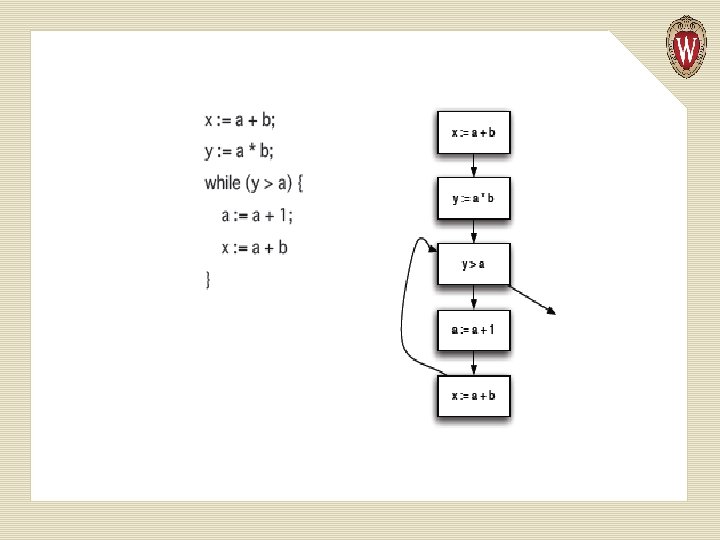
• Flow charts (also known as controlflow graphs). Nodes represent statements and conditions in a program and the edges represent potential flow of control.

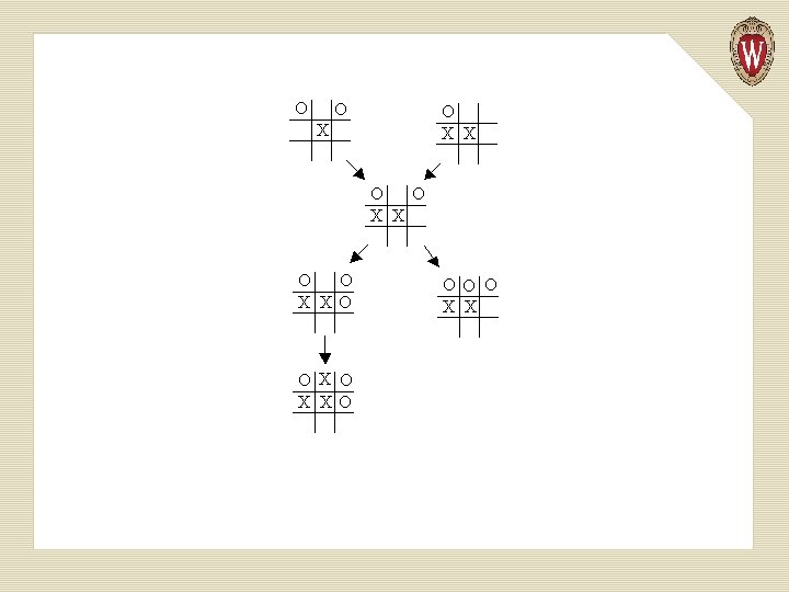
• State transition diagrams. Nodes represent states and edges represent legal moves from state to state. For example, we could use a graph to represent legal moves in a game of tic -tac-toe. Here's a small part of that graph:

Graphs can be used to answer a variety of interesting questions: • What is the cheapest way to fly from Madison to Kauai? • What are the prerequisites to CS 367? • Can variable v be used before it is initialized? • Can I force a win in tic-tac-toe given my current position?

Representing Graphs Trees are represented using a number of Treenodes, with a Tree class that points to the root node of the tree. Some graphs also have a special source or “start node. ” In such cases we use a number of Graphnodes, along with a Graph class that points to the start node.

Other graphs have no special start node, so a graph is simply a list (or set or array) of Graphnodes. Of course each Graphnode will contain data (parameterized as type T) and a list of successor nodes.

class Graphnode<T> { // *** fields *** private T data; private List<Graphnode<T>> sucessors = new Array. List<Graphnode<T>>(); // *** methods ***. . . }

public class Graph<T> { // *** fields *** private List<Graphnode<T>> nodes = new Array. List<Graphnode<T>>; // *** methods ***. . . }

What about Weighted Graphs? We need to store a weight along with the edges. We can store a list of weight, successor pairs or store a second list of edge weights.

Depth-first Search We visit nodes in the graph by following edges, with the rule that we visit “new nodes” whenever possible. Of course, not all nodes are necessarily reachable from a given start node.

Depth-first searches allow us to answer many interesting graph-related questions: • Is it connected? • Is there a path from node j to node k? • Does it contain a cycle? • What nodes are reachable from node j? • Can the nodes be ordered so that for every node j, j comes before all of its successors in the ordering?

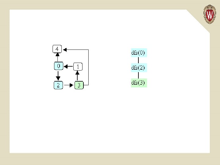
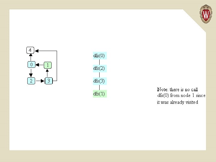
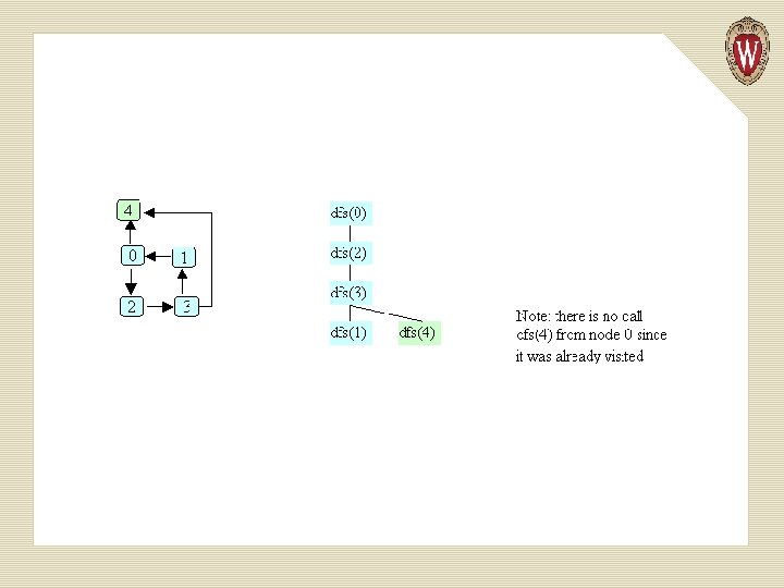
Basic Idea in Depth-first Search We keep an array of booleans called visited, one for each node. The algorithm is simply: 1. Start at node n. 2. Mark n as visited. 3. Recursively do a depth-first search from each of n’s unvisited successors.

public static void dfs (Graphnode<T> n) { n. set. Visited(true); for (Graphnode<T> m : n. get. Successors()) { if (! m. get. Visited()) { dfs(m); } } }

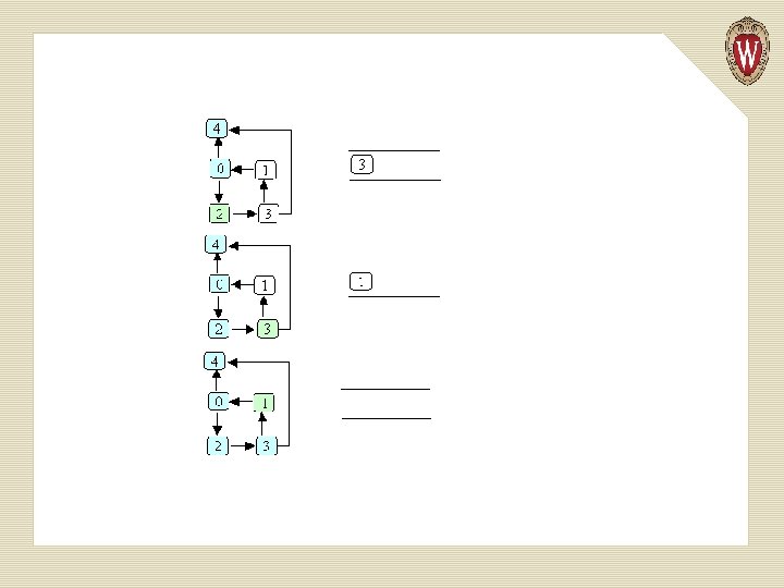
Example of Depth-first Search

Complexity of Depth-first Search We have a call for each reachable node and we examine each edge from reachable nodes. In the worst case, we may visit all nodes and edges. Complexity is O(N + E)

Uses for Depth-first Search 1. Is there a path from node j to node k? 2. What nodes are reachable from node j? 3. Is a graph connected? 4. Does a graph contain a cycle? 5. Can the nodes be ordered so that for every node j, j comes before all of its successors in the ordering?

Path Testing We want to know if a path from node j to node k exists. But our DFS algorithm already tells us this! If such a path exists, then a DFS, starting at j, will mark k as visited!

boolean path. Exists(Graphnode<T> j, Graphnode<T> k){ this. set. Visited(false); dfs(j); return k. get. Visited(); }

Reachable Nodes Here we can use our path test. We try each possible node and ask if a path from the start node exists.

Array. List<Graphnode<T>> reachable(Graphnode<T> j){ Array. List<Graphnode<T>> in = new Array. List<Graphnode<T>>(); for(Graphnode<T> k: this. get. Nodes()){ if (path. Exists(j, k) in. add(k); return in; }

Connected Graph Testing We can check where is graph is connected (or strongly connected) by simply checking if a path from each pair of nodes exists.

boolean is. Connected(){ for(Graphnode<T> j: this. get. Nodes()){ for(Graphnode<T> k: this. get. Nodes()){ if (! path. Exists(j, k) return false; } } return true; }

Cycle Detection Many graph algorithms, like reachability, assume a path of length 0 always exists from a node to itself. Thus node n is always reachable from itself by doing nothing. But a path of length 1 or more may be problematic. For example, a course may not be its own prerequisite!

Our algorithm for cycle detection will consider two cases: 1. A node n is its own immediate successor. This is possible, but also easy to test for (look at edges from n). 2. A path of length 2 or more is also possible. Here we simple look at all immediate successors of n. From each we ask if a path from that node to n exists.

boolean has. Cycle(Graphnode<T> j){ if (j. get. Sucessors(). contains(j)) return true; for (Graphnode<T> k: j. getsuccessors()){ if (path. Exists(k, j) return true; } return false; }

We may also want to know if a graph has a cycle anywhere. This is easy too – we just check each node in turn for a cycle starting at that node.

boolean has. Cycle(){ for (Graphnode<T> k: this. getnodes()){ if (has. Cycle(k)) return true; } return false; }

Topological Ordering Graphs can be used to define ordering relations among nodes. That is j → k means node j must be visited before node k is.

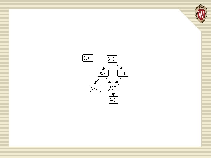
An example of ordering relations represented by graphs is a course prerequisite chain. For example:

A student may register for a course like 640 only after 537, 367, 354 and 302 have been taken. However 310 may be taken before or after 640, since no ordering between them is indicated.

A topological ordering of nodes in a graph is a sequencing of nodes that respects the graph’s ordering relations. That is, if the graph contains j → k, then j must always be listed before k. We can use a variant of depth-first search to do a topological ordering. We require that the graph we will order has no cycles. Cycles make a valid numbering impossible. Why?

Recall that we already know for to test a graph for cycles. We will identify one or more “start nodes” in a graph. A start node is simply a node that has no incoming edges. We start at such nodes because starting elsewhere makes them unreachable. Each node has a boolean flag is. Done, initially false. When a node’s is. Done flag becomes true, it is assigned an ordering number and needs no further processing.

As in depth first search, we process a node after all its children have been processed. Thus leaf nodes get a number, then their parents, etc. We assign numbers last to first so that the order number assigned to a leaf is larger than that assigned to its parent.

The method we will use is int top. Order(Graphnode<T> n, int num) The parameter num is the last (highest) number to be assigned. The method returns the highest unused order number (the graph may not be connected, so numbering may need to be done in pieces).

int top. Order(Graphnode<T> n, int num) { for (Graphnode<T> m : n. get. Successors()) { if (! m. is. Done) { num = top. Order(m, num); } } // here when n has no more successors n. is. Done = true; n. set. Order(num); return num - 1; }

Example of top. Order We order the course prerequisite graph We’ll start at node 302 with num = 7.

Breadth-first Search An alternative to depth-first choice is breadth-first search. From a starting node all nodes at distance one are visited, then nodes at distance 2, etc. This sort of search is used to find the shortest path between two nodes.

We’ve already seen the tree-oriented version of breadth-first search – level order traversal. As in level-order traversal, we use a queue to remember nodes waiting to be fully processed. We also use a “visited” flag to remember nodes already processed (and queued).

public void bfs(Graphnode<T> n) { Queue<Graphnode> queue = new Queue<Graphnode>(); n. set. Visited(true); queue. enqueue( n ); while (!queue. is. Empty())) { Graphnode<T> current = queue. dequeue(); for (Graphnode<T> k : current. get. Successors()) { if (! k. get. Visited()){ k. set. Visited(true); queue. enqueue(k); } // end if k not visited } // end for every successor k } // end while queue not empty }

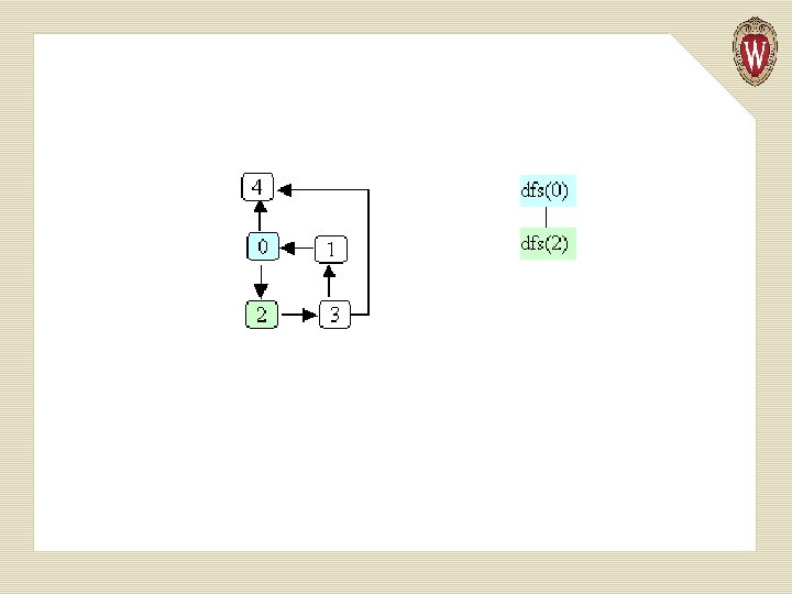
Example of Breadth-first Search

Starting at node 0, the visit order is

Shortest Path We can use bfs to find the shortest distance to each reachable node: • add a distance field to each node • when bfs is called with node n, set n's distance to zero • when a node k is about to be enqueued, set k's distance to the distance of the current node (the one that was just dequeued) + 1

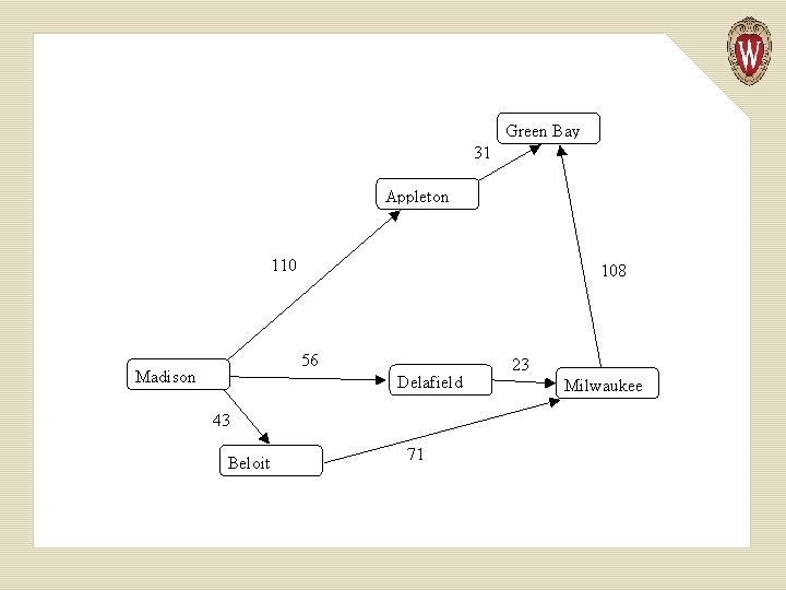
Shortest Weighted Path The shortest path does not always give us the best result. Consider a highway map, listing cities and distances:

Shortest path tells us the best route from Madison to Milwaukee is through Beloit, since it takes just “two steps. ” But looking at distances tells us the route through Delafield is better. What we need is a shortest weighted path algorithm. Dijkstra’s algorithm lets us compute shortest weighted paths efficiently.

Dijkstra’s Algorithm Dijkstra’s algorithm uses an “explorer” approach, in which we visit nodes along various paths, always recording the shortest (or fastest, or cheapest) distance. We start at a source node. The distance from source s to itself is trivially 0.

We then look at nodes one step away from the source. Tentative distances are recorded. The smallest distance gives us the shortest path from s to one node. Why? This node is marked as “finished. ” We next look the nearest node not marked as finished. Its successors are explored. The node marked with the shortest distance is marked as finished. Then the unfinished node with the shortest distance is explored.

The process continues until all nodes are marked as finished. Here is an outline of Dijkstra’s Algorithm. We start with: A graph, G, with edges E of the form (v 1, v 2) and vertices (nodes) V, and a source vertex, s.

The data structures we use are: dist : array of distances from the source to each vertex prev : array of pointers to preceding vertices i : loop index F : list of finished vertices U : list or heap unfinished vertices

Initialization: F = Empty list U = All vertices (nodes) for (i = 0 ; i < U. size(); i++) { dist[i] = INFINITY; prev[i] = NULL; } dist[s] = 0; // Starting node

while (U. size() > 0) { pick the vertex, v, in U with the shortest path to s; add v to F; remove v from U; for each edge of v, (v 1, v 2) { if (dist[v 1] + length(v 1, v 2) < dist[v 2]) { dist[v 2] = dist[v 1] + length(v 1, v 2); prev[v 2] = v 1; } } }

Example of Dijkstra’s Algorithm

Complexityof Dijkstra’s Algorithm The complexity is measured in terms of edges (E) and vertices (nodes) N. If list U is implemented as an unordered list, execution time is O(N 2) Why? As each node is processed, the U list must be searched for the cheapest unfinished node.

But the U list may also be implemented as a priority queue (using a heap). Then getting the cheapest unfinished node is only log N. But each time an edge is used to update the best known distance, the priority queue may need to be restructured into heap form. This leads to O(E log N), which is usually better than O(N 2).

Traveling Salesman Problem Given n cities we wish the shortest (or fastest, or cheapest) path that visits each city and returns to the starting point.

The obvious approach is to try all possible paths. But this is exponential! Perhap a generalization of Dijkstra’s algorithm? No – theoretical computer science tells us the best we can do most likely must be exponential.

Approximation Algorithms What if we accept something close to optimal? • Christofis’s algorithm guarantees a solution no worst than 50% above optimal. It is O(N 3). • Heuristics often improve Christofis’s bound. For example, try to swap pairs of adjacent cities.

CS 577 Introduction to Algorithms Basic paradigms for the design and analysis of efficient algorithms: greed, divide-and-conquer, dynamic programming, reductions, and the use of randomness. Computational intractability including typical NPcomplete problems and ways to deal with them.

q No Office Hours Wed and Thurs q Today’s topics: u Graphs u Depth-First Search u Graph Algorithms