Data Structures Algorithms Lecture 6 Graph Algorithms Data

Data Structures & Algorithms Lecture # 6 Graph Algorithms

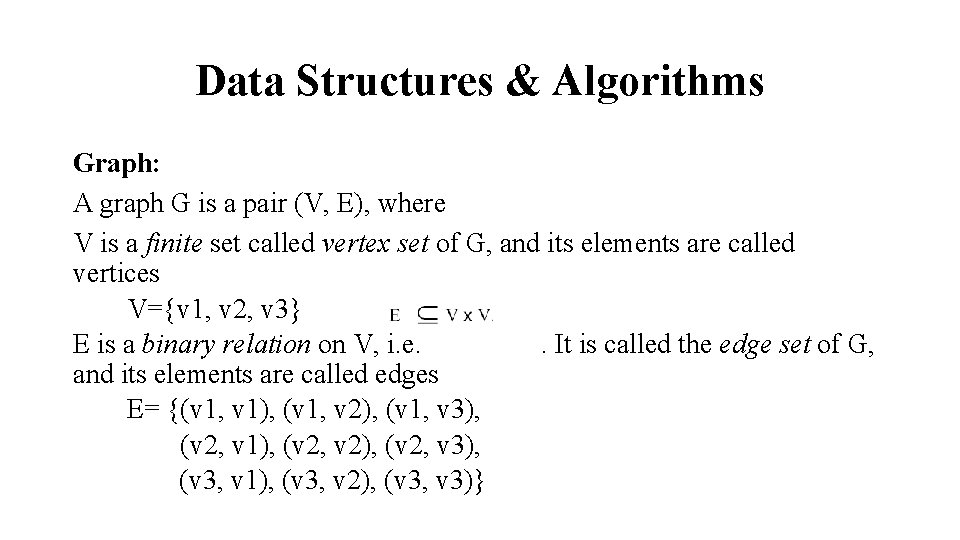
Data Structures & Algorithms Graph: A graph G is a pair (V, E), where V is a finite set called vertex set of G, and its elements are called vertices V={v 1, v 2, v 3} E is a binary relation on V, i. e. . It is called the edge set of G, and its elements are called edges E= {(v 1, v 1), (v 1, v 2), (v 1, v 3), (v 2, v 1), (v 2, v 2), (v 2, v 3), (v 3, v 1), (v 3, v 2), (v 3, v 3)}

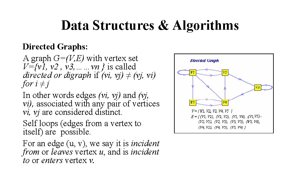
Data Structures & Algorithms Directed Graphs: A graph G=(V, E) with vertex set V={v 1, v 2 , v 3, ……vn } is called directed or digraph if (vi, vj) ≠ (vj, vi) for i ≠ j In other words edges (vi, vj) and (vj, vi), associated with any pair of vertices vi, vj are considered distinct. Self loops (edges from a vertex to itself) are possible. For an edge (u, v), we say it is incident from or leaves vertex u, and is incident to or enters vertex v.

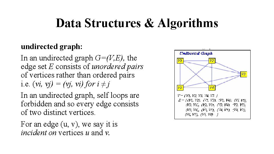
Data Structures & Algorithms undirected graph: In an undirected graph G=(V, E), the edge set E consists of unordered pairs of vertices rather than ordered pairs i. e. (vi, vj) = (vj, vi) for i ≠ j In an undirected graph, self loops are forbidden and so every edge consists of two distinct vertices. For an edge (u, v), we say it is incident on vertices u and v.

Data Structures & Algorithms Adjacency: If (u, v) is an edge in a graph G=(V, E), we say vertex v is adjacent to vertex u. When graph is undirected, the adjacency relationship is symmetric. When graph is directed, the adjacency relationship is not necessarily symmetric. If v is adjacent to u in a directed graph, we say u → v.

Data Structures & Algorithms Complete Graphs: A graph in which every pair of vertices is adjacent is called a complete graph. In other words, a graph which has all the edges is referred to as complete. An undirected complete graph , with n vertices, has n(n-1)/2 edges. Its space complexity is O(n 2). Such a graph is called dense. A complete directed graph with n vertices has n 2 edges, including edges associated with all individual vertices. If individual edges are excluded, the total number of edges is n(n-1).

Data Structures & Algorithms Degree: In an undirected graph, the number of edges incident on a vertex is called the degree of a vertex. A vertex with degree 0 is said to be isolated. In a directed graph, the out-degree of a vertex is the number of edges leaving it. In a directed graph, the in-degree of a vertex is the number of edges entering it. In a directed graph, the degree of a vertex is the in-degree + the outdegree.

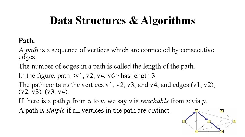
Data Structures & Algorithms Path: A path is a sequence of vertices which are connected by consecutive edges. The number of edges in a path is called the length of the path. In the figure, path <v 1, v 2, v 4, v 6> has length 3. The path contains the vertices v 1, v 2, v 3, and v 4, and edges (v 1, v 2), (v 2, v 3), (v 3, v 4). If there is a path p from u to v, we say v is reachable from u via p. A path is simple if all vertices in the path are distinct.

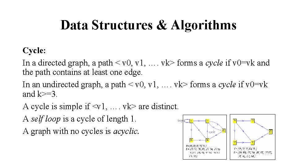
Data Structures & Algorithms Cycle: In a directed graph, a path < v 0, v 1, …. vk> forms a cycle if v 0=vk and the path contains at least one edge. In an undirected graph, a path < v 0, v 1, …. vk> forms a cycle if v 0=vk and k>=3. A cycle is simple if <v 1, …. vk> are distinct. A self loop is a cycle of length 1. A graph with no cycles is acyclic.

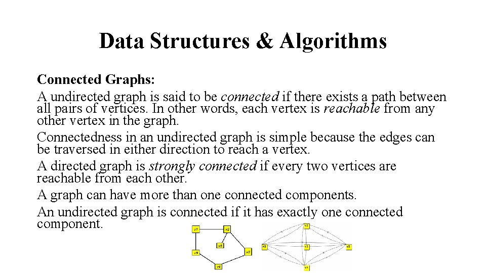
Data Structures & Algorithms Connected Graphs: A undirected graph is said to be connected if there exists a path between all pairs of vertices. In other words, each vertex is reachable from any other vertex in the graph. Connectedness in an undirected graph is simple because the edges can be traversed in either direction to reach a vertex. A directed graph is strongly connected if every two vertices are reachable from each other. A graph can have more than one connected components. An undirected graph is connected if it has exactly one connected component.

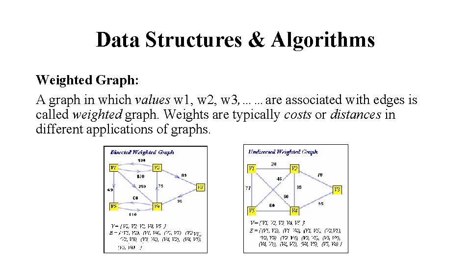
Data Structures & Algorithms Weighted Graph: A graph in which values w 1, w 2, w 3, ……are associated with edges is called weighted graph. Weights are typically costs or distances in different applications of graphs.

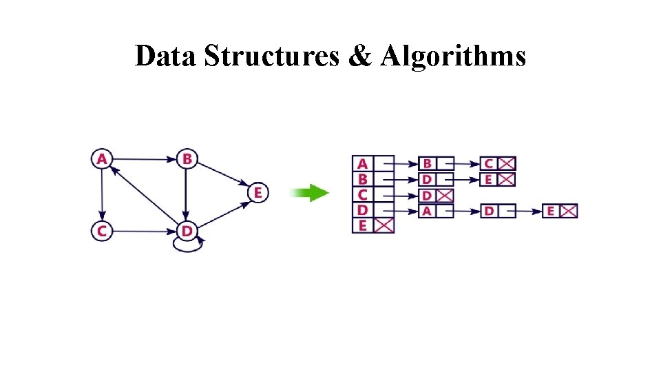
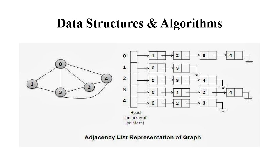
Data Structures & Algorithms Graph Representation: Two standard ways to represent directed and undirected graphs • Adjacency list • Adjacency matrix The list representation consists of an array of linked lists, each corresponding to a vertex. The list stores all of the vertices that are linked to a given vertex. Let G=(V, E) be a graph. For each u V, the adjacency list Adj(u) contains all the vertices v such that there is an edge (u , v ) E. Vertices in an adjacency list are typically stored in an arbitrary order.

Data Structures & Algorithms

Data Structures & Algorithms

Data Structures & Algorithms Advantages and Disadvantages: Usually preferred because it provides a compact way to represent sparse graphs – those for which |E| is much less that |V|2 For both directed and undirected graphs, the amount of representation required is θ(V+E). Can be readily adapted to represent weighted graphs. The weight is simply stored with vertex v in u’s adjacency list. There is no quicker way to determine if a given edge (u, v) is present in the graph than to search for v in the adjacency list Adj[u]

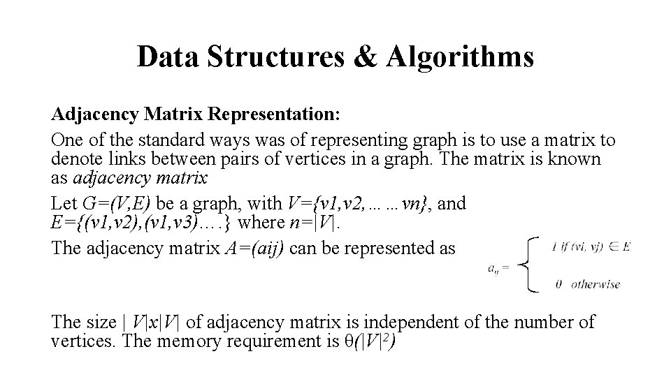
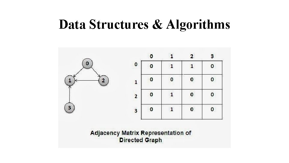
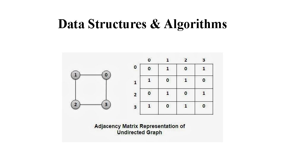
Data Structures & Algorithms Adjacency Matrix Representation: One of the standard ways was of representing graph is to use a matrix to denote links between pairs of vertices in a graph. The matrix is known as adjacency matrix Let G=(V, E) be a graph, with V={v 1, v 2, ……vn}, and E={(v 1, v 2), (v 1, v 3)…. } where n=|V|. The adjacency matrix A=(aij) can be represented as The size | V|x|V| of adjacency matrix is independent of the number of vertices. The memory requirement is θ(|V|2)

Data Structures & Algorithms

Data Structures & Algorithms

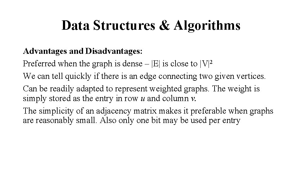
Data Structures & Algorithms Advantages and Disadvantages: Preferred when the graph is dense – |E| is close to |V|2 We can tell quickly if there is an edge connecting two given vertices. Can be readily adapted to represent weighted graphs. The weight is simply stored as the entry in row u and column v. The simplicity of an adjacency matrix makes it preferable when graphs are reasonably small. Also only one bit may be used per entry

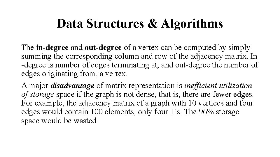
Data Structures & Algorithms The in-degree and out-degree of a vertex can be computed by simply summing the corresponding column and row of the adjacency matrix. In -degree is number of edges terminating at, and out-degree the number of edges originating from, a vertex. A major disadvantage of matrix representation is inefficient utilization of storage space if the graph is not dense, that is, there are fewer edges. For example, the adjacency matrix of a graph with 10 vertices and four edges would contain 100 elements, only four 1’s. The 96% storage space would be wasted.

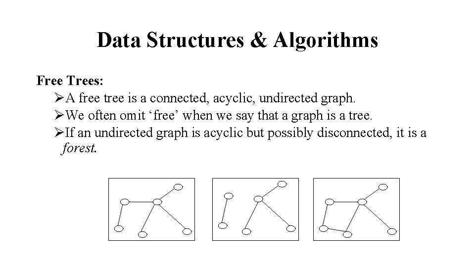
Data Structures & Algorithms Free Trees: ØA free tree is a connected, acyclic, undirected graph. ØWe often omit ‘free’ when we say that a graph is a tree. ØIf an undirected graph is acyclic but possibly disconnected, it is a forest.

Data Structures & Algorithms Properties of Free Trees: Let G=(V, E) be an undirected graph. The following statements are equivalent: ØG is a free tree ØAny two vertices in G are connected by a unique simple path ØG is connected, but if any edge is removed from E, the resulting graph is disconnected ØG is connected and |E|=|V|-1 ØG is acyclic, but if any edge is added to E, the resulting graph contains a cycle

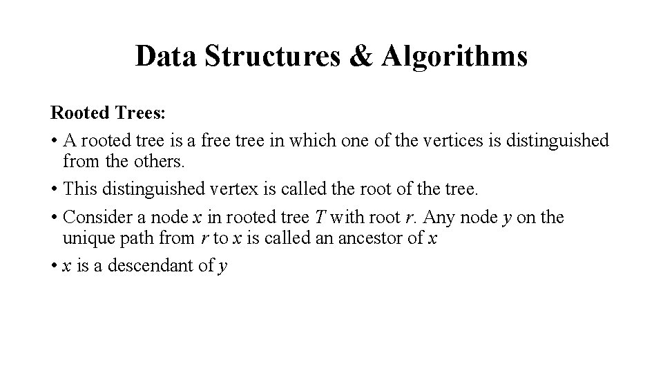
Data Structures & Algorithms Rooted Trees: • A rooted tree is a free tree in which one of the vertices is distinguished from the others. • This distinguished vertex is called the root of the tree. • Consider a node x in rooted tree T with root r. Any node y on the unique path from r to x is called an ancestor of x • x is a descendant of y

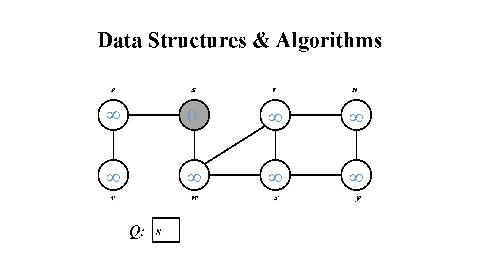
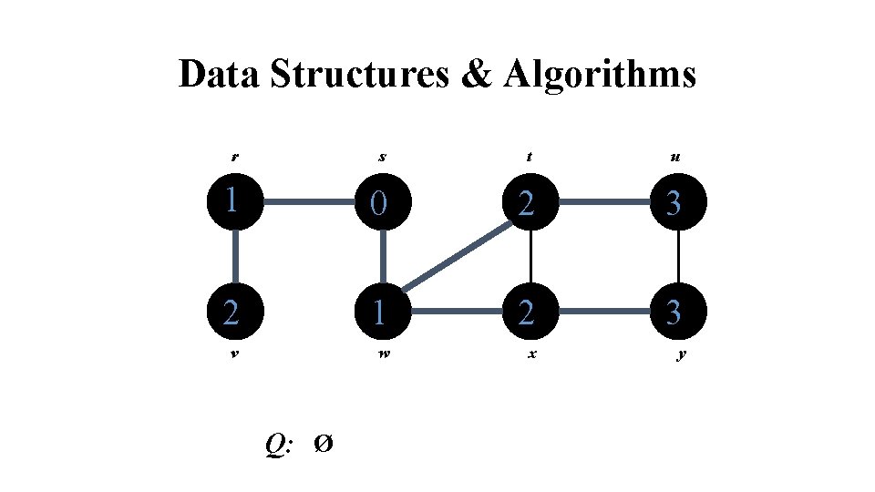
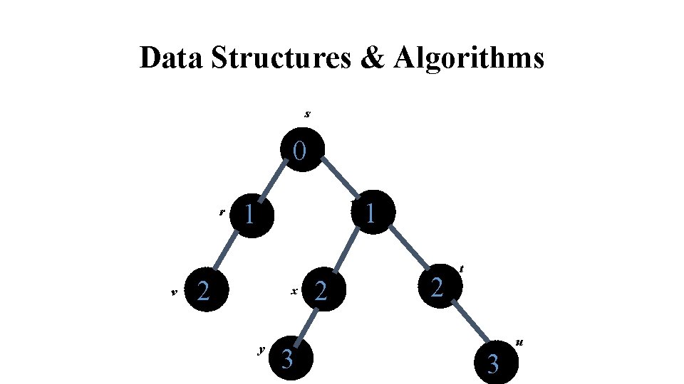
Data Structures & Algorithms Breadth First Search: The Breadth First Search (BFS) is one of the simplest graph traversal methods. The method proceeds by visiting all immediate neighbors (vertices one edge away) of a source vertex s, then visiting neighbor’s neighbors (vertices two edges away), and so forth, until all reachable vertices have been visited. Each node is visited once only. It produces a breadth-first tree with root s that contains all reachable vertices. Note: might also build a forest if graph is not connected

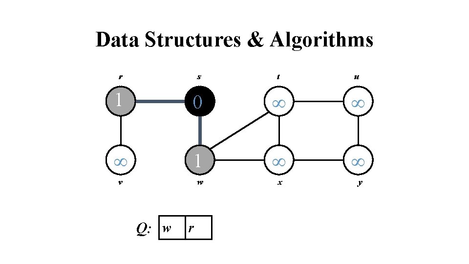
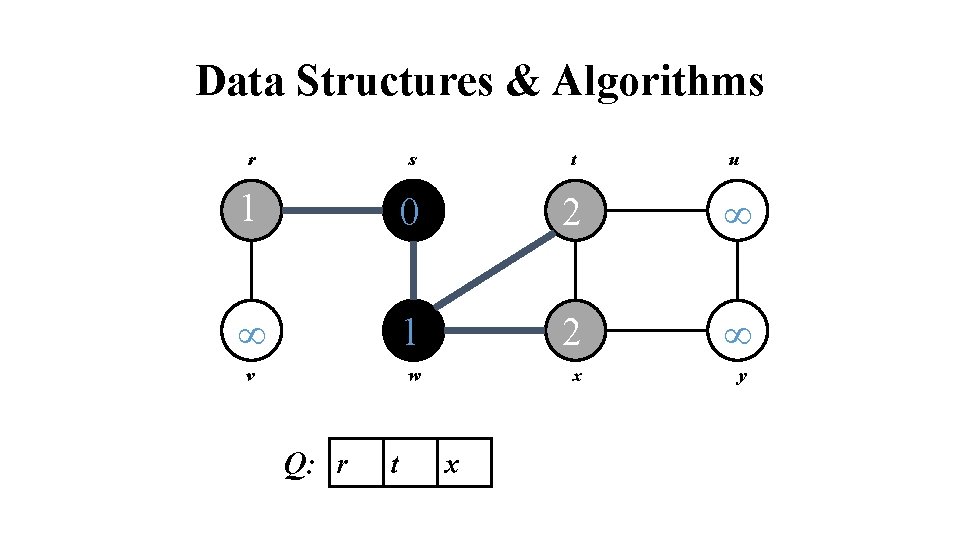
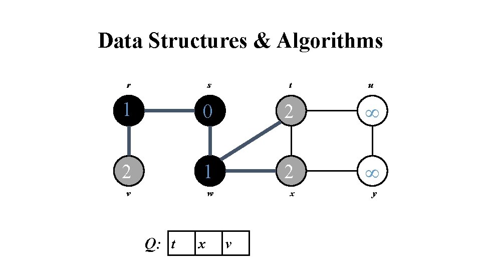
Data Structures & Algorithms For any vertex v reachable from s, the path in the BFS tree from s to v corresponds to a ‘shortest path’ from s to v in G, i. e. a path containing smallest number of edges. The algorithm works for directed and undirected graphs. A queue is used to implement the BFS procedure. It keeps track of vertices to be visited next. A vertex insert into the queue is said to be in ready state. An enqueued vertex is said be in wait state. The dequeued vertex is referred to as processed.

Data Structures & Algorithms Will associate vertex “colors” to guide the algorithm ØWhite vertices have not been discovered, All vertices start out white. ØGrey vertices are discovered but not fully explored. They may be adjacent to white vertices. ØBlack vertices are discovered and fully explored. They are adjacent only to black and gray vertices. Explore vertices by scanning adjacency list of grey vertices

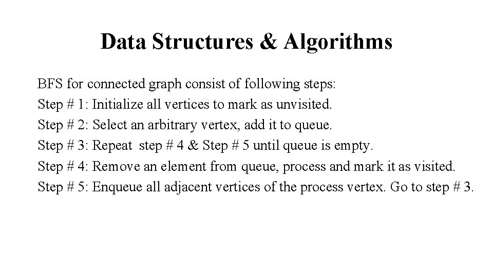
Data Structures & Algorithms BFS for connected graph consist of following steps: Step # 1: Initialize all vertices to mark as unvisited. Step # 2: Select an arbitrary vertex, add it to queue. Step # 3: Repeat step # 4 & Step # 5 until queue is empty. Step # 4: Remove an element from queue, process and mark it as visited. Step # 5: Enqueue all adjacent vertices of the process vertex. Go to step # 3.

Data Structures & Algorithms BFS(G, s) for each vertex u ϵ V[G] –{s} do color[u] ← white d[u] ← ∞ π[u] ← NIL color[s] ← gray d[s] ← 0 π[s] ← NIL Q←Ø ENQUEUE(Q, s) While Q ≠ Ø do u ← DEQUEUE(Q) for each v ϵ Adj[u] do if color[v] = white then color[v] ← gray d[v] ← d[u] + 1 π[v] ← u ENQUEUE(Q, v) color[u] ← BLACK

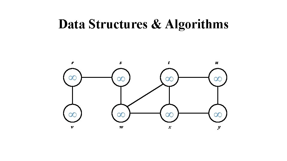
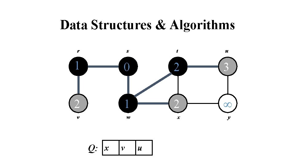
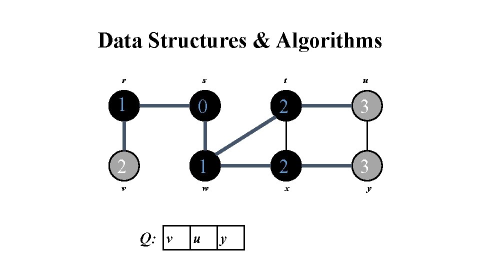
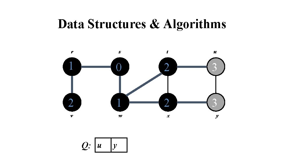
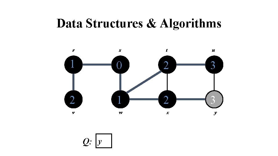
Data Structures & Algorithms lines 1– 4 paint every vertex white, set d[u] to be infinity for each vertex u, and set the parent of every vertex to be NIL. Line 5 paints s gray, since we consider it to be discovered as the procedure begins. Line 6 initializes d[s] to 0, and line 7 sets the predecessor of the source to be NIL. Lines 8– 9 initialize Q to the queue containing just the vertex s. The while loop of lines 10– 18 iterates as long as there remain gray vertices, which are discovered vertices that have not yet had their adjacency lists fully examined.

Data Structures & Algorithms r s t u v w x y

Data Structures & Algorithms r s t u 0 v w x y Q: s

Data Structures & Algorithms r s t u 1 0 1 v w x y Q: w r

Data Structures & Algorithms r s t u 1 0 2 1 2 v w x Q: r t x y

Data Structures & Algorithms r s t u 1 0 2 2 1 2 v w x Q: t x v y

Data Structures & Algorithms r s t u 1 0 2 3 2 1 2 v w x Q: x v u y

Data Structures & Algorithms r s t u 1 0 2 3 2 1 2 3 v w x y Q: v u y

Data Structures & Algorithms r s t u 1 0 2 3 2 1 2 3 v w x y Q: u y

Data Structures & Algorithms r s t u 1 0 2 3 2 1 2 3 v w x y Q: y

Data Structures & Algorithms r s t u 1 0 2 3 2 1 2 3 v w x y Q: Ø

Data Structures & Algorithms s 0 r v w 1 2 x y 3 2 1 2 t 3 u

Data Structures & Algorithms BFS calculates the shortest-path distance to the source node Shortest-path distance (s, v) = minimum number of edges from s to v, or if v not reachable from s. BFS builds breadth-first tree, in which paths to root represent shortest paths in G. The results of BFS may depend on order in which the neighbors of a given tree are visited. The BFS tree may vary, but the distances d computed by the algorithm will not.

Data Structures & Algorithms Analysis of Breadth First Search: The running time for BFS consists of following major components • Ti =Initializing vertices T • Tq =Queuing and Dequeuing • Ts = Scanning Adjacency list The Graph G(V, E) has |V| vertices and |E| edges. Each vertex is initialized once. Therefore, Ti = O(V) The queuing and dequeuing operations take O(1) time, and each vertex is queued and dequeued once, • Tq =O(V)

Data Structures & Algorithms The scanning of Adjacency list takes place for each vertex. In worst case all links are examined. The total time is proportional to the number of edges scanned. Since |E| is the number of edges in G, • Ts =O(E) Thus time running time is given by O(|V|+|E|)

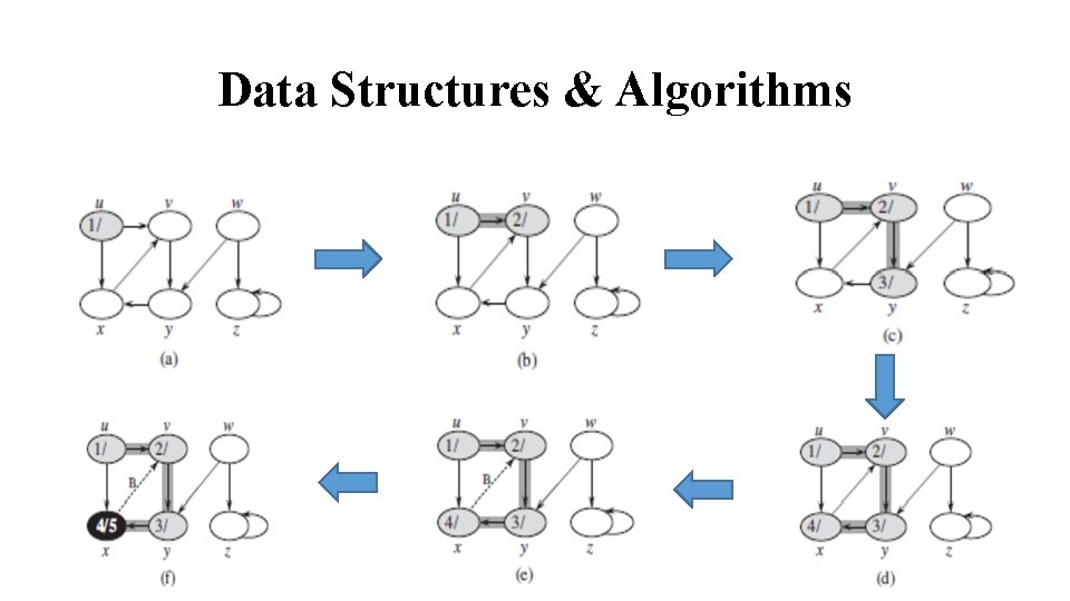
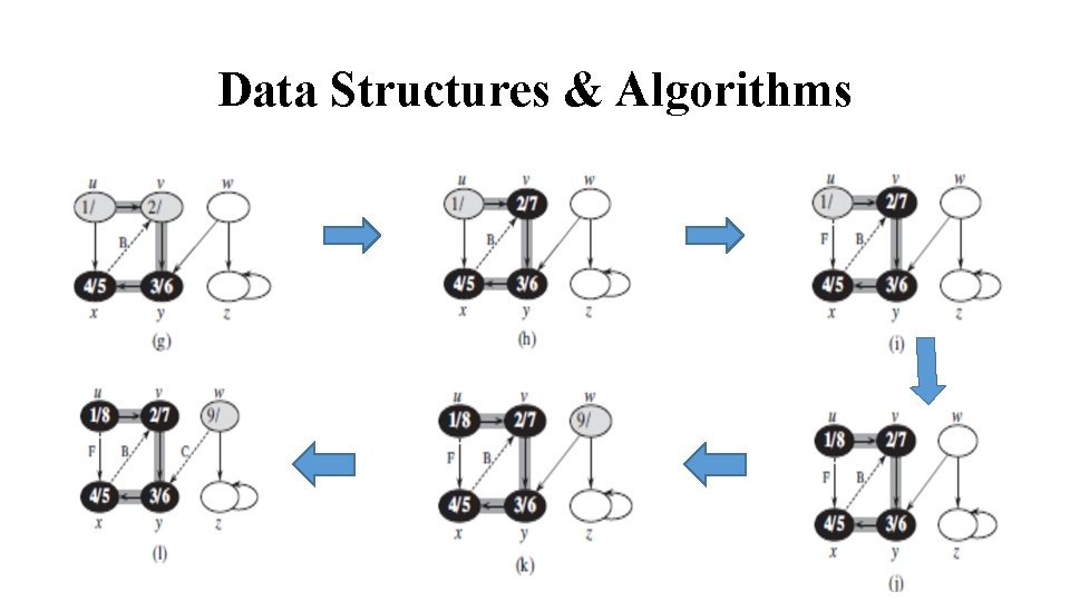
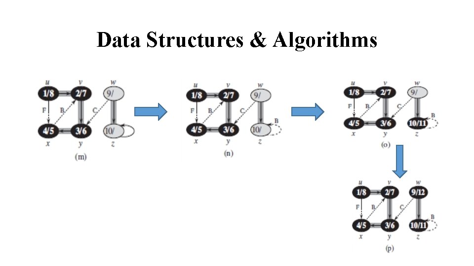
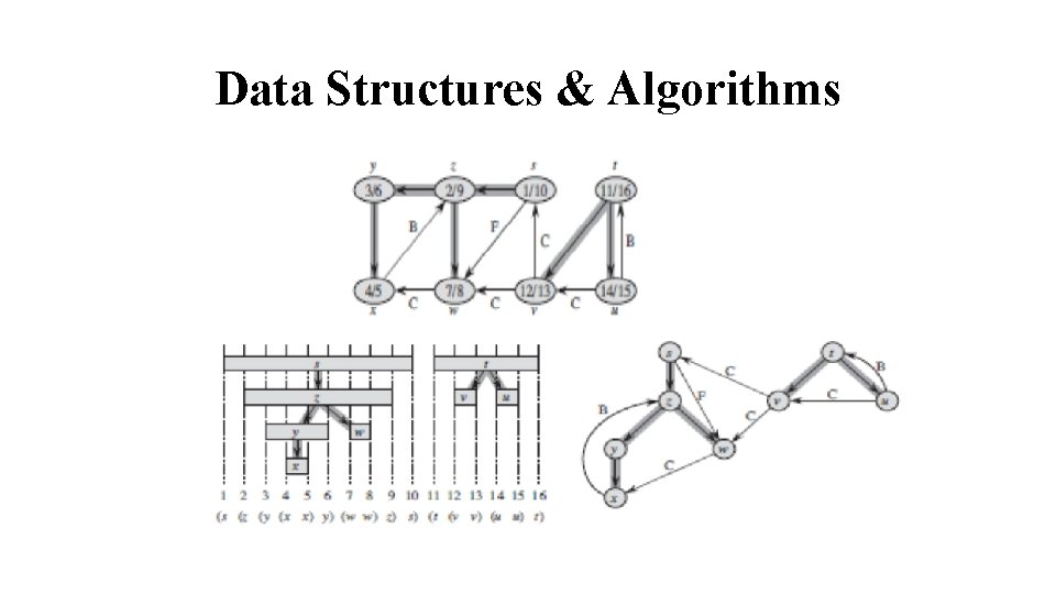
Data Structures & Algorithms Depth First Search: ØThe Depth First Search (DFS) is one of the standard graph traversal methods. ØEach node is visited once only. ØThe method proceeds by searching deeper in the graph wherever possible. ØEdges are discovered out of the most recently discovered vertex v that still has unexplored edges leaving it.

Data Structures & Algorithms ØWhen all of v’s edges have been explored, the search back tracks to explore edges leaving the vertex from which v was discovered. ØIn DFS, the search may be repeated from multiple sources ØIf a graph has any sub-graph (which is not reachable from the initial vertex), the procedure is re-started by choosing a vertex from the unvisited sub-graph.

Data Structures & Algorithms FS for connected graph consist of following steps: Step # 1: Initialize all vertices to mark as unvisited. Step # 2: Select an arbitrary vertex, add it to queue. Step # 3: Repeat step # 4 & Step # 5 until queue is empty. Step # 4: Remove an element from queue, process and mark it as visited. Step # 5: Enqueue all adjacent vertices of the process vertex. Go to step # 3.

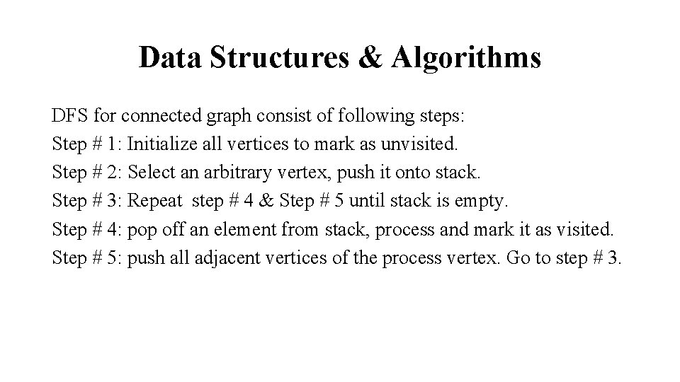
Data Structures & Algorithms DFS for connected graph consist of following steps: Step # 1: Initialize all vertices to mark as unvisited. Step # 2: Select an arbitrary vertex, push it onto stack. Step # 3: Repeat step # 4 & Step # 5 until stack is empty. Step # 4: pop off an element from stack, process and mark it as visited. Step # 5: push all adjacent vertices of the process vertex. Go to step # 3.

Data Structures & Algorithms

Data Structures & Algorithms

Data Structures & Algorithms

Data Structures & Algorithms

Data Structures & Algorithms

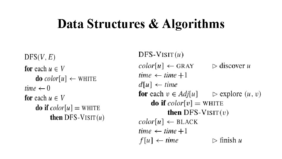
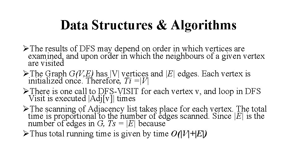
Data Structures & Algorithms ØThe results of DFS may depend on order in which vertices are examined, and upon order in which the neighbours of a given vertex are visited ØThe Graph G(V, E) has |V| vertices and |E| edges. Each vertex is initialized once. Therefore, Ti =|V| ØThere is one call to DFS-VISIT for each vertex v, and loop in DFS Visit is executed |Adj[v]| times ØThe scanning of Adjacency list takes place for each vertex. The total time is proportional to the number of edges scanned. Since |E| is the number of edges in G, Ts = |E| because ØThus total running time is given by time O(|V|+|E|)

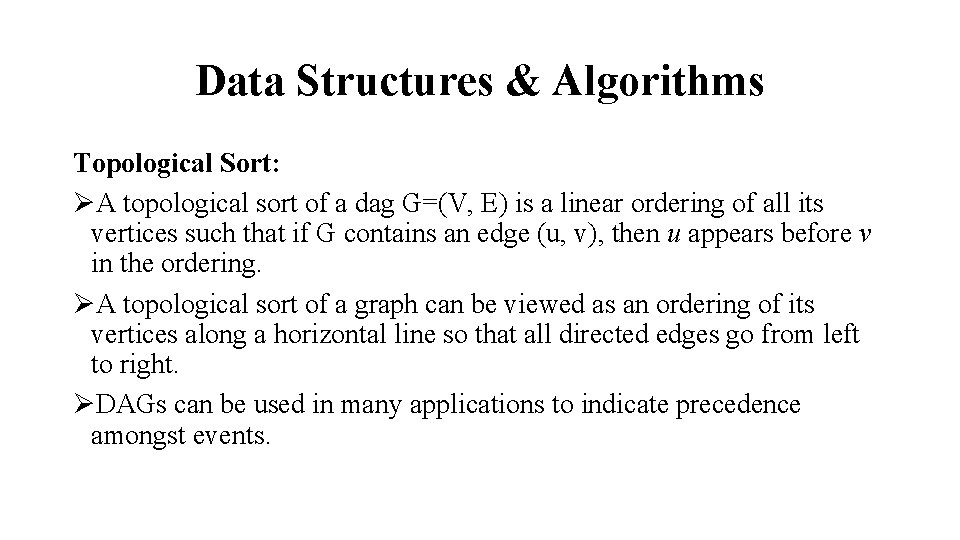
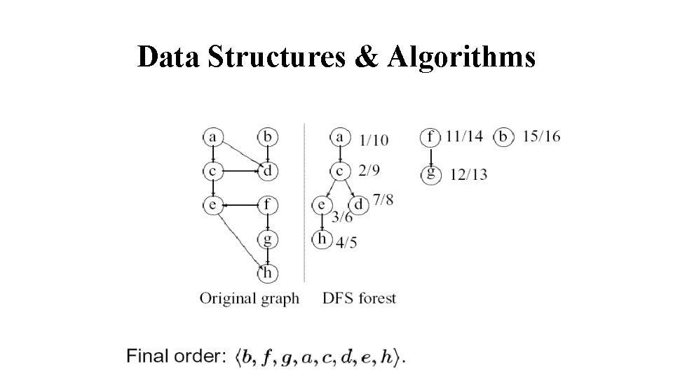
Data Structures & Algorithms Topological Sort: ØA topological sort of a dag G=(V, E) is a linear ordering of all its vertices such that if G contains an edge (u, v), then u appears before v in the ordering. ØA topological sort of a graph can be viewed as an ordering of its vertices along a horizontal line so that all directed edges go from left to right. ØDAGs can be used in many applications to indicate precedence amongst events.

Data Structures & Algorithms Topological-Sort(G) 1. Call DFS(G) to compute finishing times f[v] for each vertex v 2. As each vertex is finished, insert it onto the front of a linked list 3. Return the linked list of vertices Topological sort can be performed in time O(|V|+|E|)

Data Structures & Algorithms