Data Structures and Algorithms in Parallel Computing Lecture

Data Structures and Algorithms in Parallel Computing Lecture 1

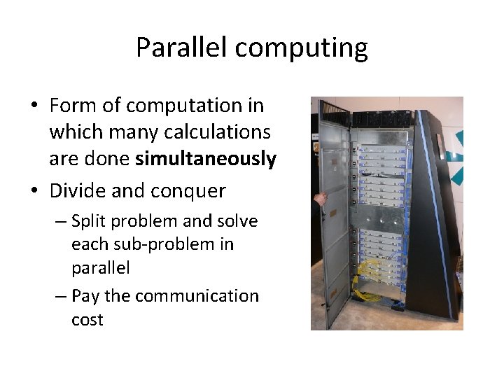
Parallel computing • Form of computation in which many calculations are done simultaneously • Divide and conquer – Split problem and solve each sub-problem in parallel – Pay the communication cost

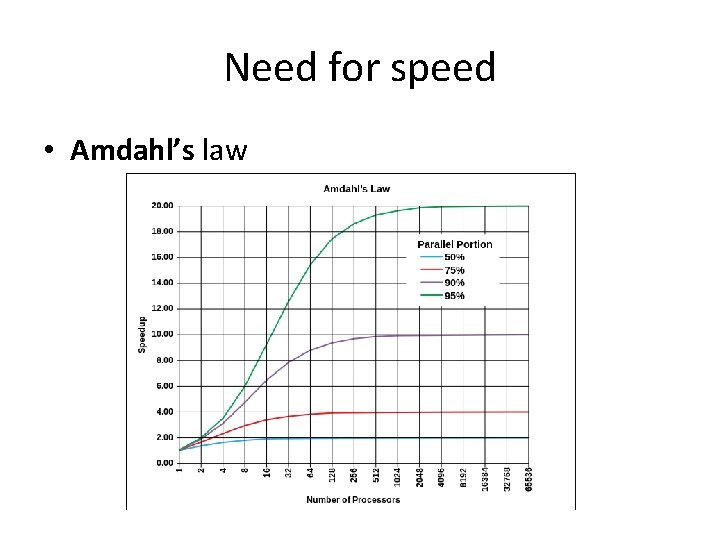
A bit of history • 1958 – S. Gill discusses parallel programming – J. Cocke and D. Slotnick discuss parallel numerical computing • 1967 – Amdahl’s law is introduced • Defines the speed-up due to parallelism • 1969 – Honneywell introduces the first symmetric multiprocessor • It allowed for up to 8 parallel processors • June 2016 – China’s Sunway Taihu. Light is the fastest computer in the world • 93 petaflops

Classification • Bit level – Increase word size to reduce number of instructions • 2 instructions to add a 16 bit number on 8 bit processor • 1 instruction to add a 16 bit number on 16 bit processor • Instruction level – Hardware level – Software level – Example 1. e = a + b 2. f = c + d 3. m = e * f • #3 depends on #1 and #2 both of which can be executed in parallel

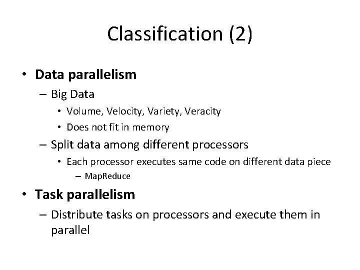
Classification (2) • Data parallelism – Big Data • Volume, Velocity, Variety, Veracity • Does not fit in memory – Split data among different processors • Each processor executes same code on different data piece – Map. Reduce • Task parallelism – Distribute tasks on processors and execute them in parallel

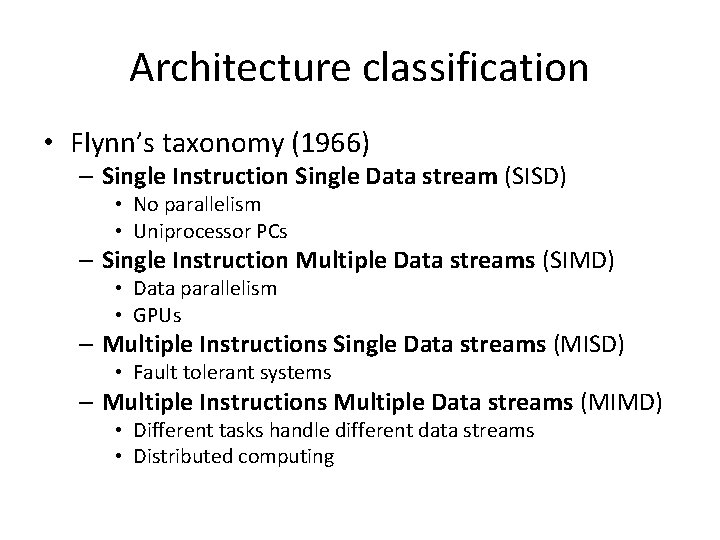
Architecture classification • Flynn’s taxonomy (1966) – Single Instruction Single Data stream (SISD) • No parallelism • Uniprocessor PCs – Single Instruction Multiple Data streams (SIMD) • Data parallelism • GPUs – Multiple Instructions Single Data streams (MISD) • Fault tolerant systems – Multiple Instructions Multiple Data streams (MIMD) • Different tasks handle different data streams • Distributed computing

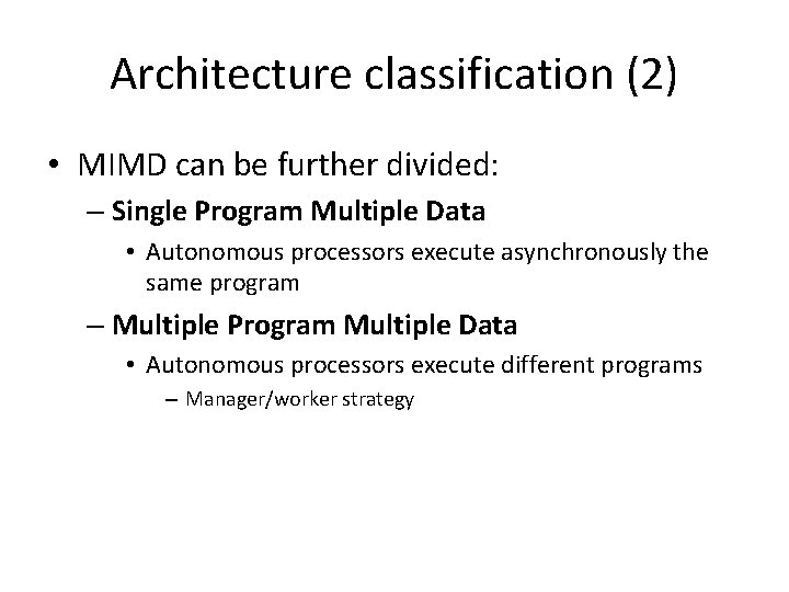
Architecture classification (2) • MIMD can be further divided: – Single Program Multiple Data • Autonomous processors execute asynchronously the same program – Multiple Program Multiple Data • Autonomous processors execute different programs – Manager/worker strategy

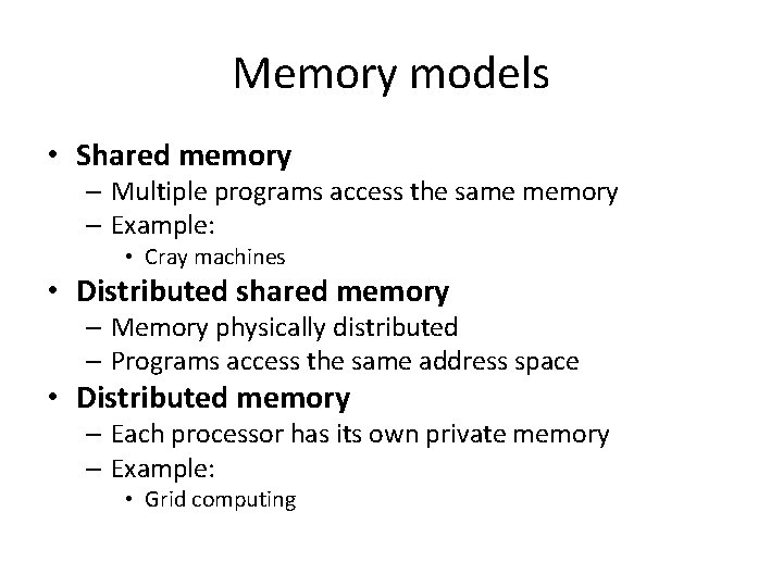
Memory models • Shared memory – Multiple programs access the same memory – Example: • Cray machines • Distributed shared memory – Memory physically distributed – Programs access the same address space • Distributed memory – Each processor has its own private memory – Example: • Grid computing

Need for speed • Amdahl’s law

Algorithm design How to transform a sequential algorithm in a parallel one? Example: Compute the sum of n numbers – Numbers are stored in a matrix A 1. Pair A[i] with A[i+1] 2. Add the pair on machine k • • We need n/k machines We obtain a new sequence of n/k numbers 3. Repeat from step 1 After log 2 n iterations we get a sequence of 1 number: the sum

Modeling parallel computations • No consensus on the right model • Random-Access Machine (RAM) – Ignores many of the computer architecture details – Captures enough detail for reasonable accuracy – Each CPU operation including arithmetic and logical operations, and memory accesses requires 1 time step

Multiprocessor model • Local memory – Each processor has its own local memory – Processors are attached to a local network • Modular memory – M memory modules • Parallel RAM (PRAM) – Shared memory – No real machine lives up to its ideal of unit time access to a shared memory – Where can it be implemented? FPGAs (SRAM)

Network limitations Communication bottlenecks • Bus topology – Processors take turn to access the bus • 2 dimensional mesh – Remote accesses are done by routing messages – Appears in local memory machines • Multistage network – Used to connect one set of input switches to another set of output switches – Designed for telephone networks – Appears in modular memory machines – Processors are attached to input switches and memory to output switches

Network limitations (2) Algorithms designed for one topology may not work for another! Algorithms considering network topology are more complicated than the ones designed for simpler models such as PRAM

Model routing capabilities • Alternative to topology modeling • Consider – Bandwidth • Rate at which a processor can inject data in the network – Latency • Time to traverse the network

Model routing capabilities (2) • Existing models: – Postal model • Model only latency – Bulk Synchronous Parallel • Adds g, i. e. , the minimum ratio of computation steps to communication steps – Log. P • Adds o, i. e. , the overhead of a processor upon sending/receiving a message

Primitive operations • Basic operations that processors and network can perform – All processors can perform the same local instructions as the single processor in the RAM model – Processors can also issue non-local memory requests • For message passing • For global operations

Restrictions on operations • Restrictions on operations can exist – E. g. , two processors may not write the same memory location at the same time • Exclusive vs. concurrent access – Exclusive read exclusive write (EREW) – Concurrent read concurrent write (CRCW) – Concurrent read exclusive write (CREW) • Solving concurrent writes – Random picking – Priority picking – Queued access: Queued read queued write

Examples of operations • Read-write to non-local memory or other processors • Synchronization • Broadcast messages to processors • Gather messages from processors

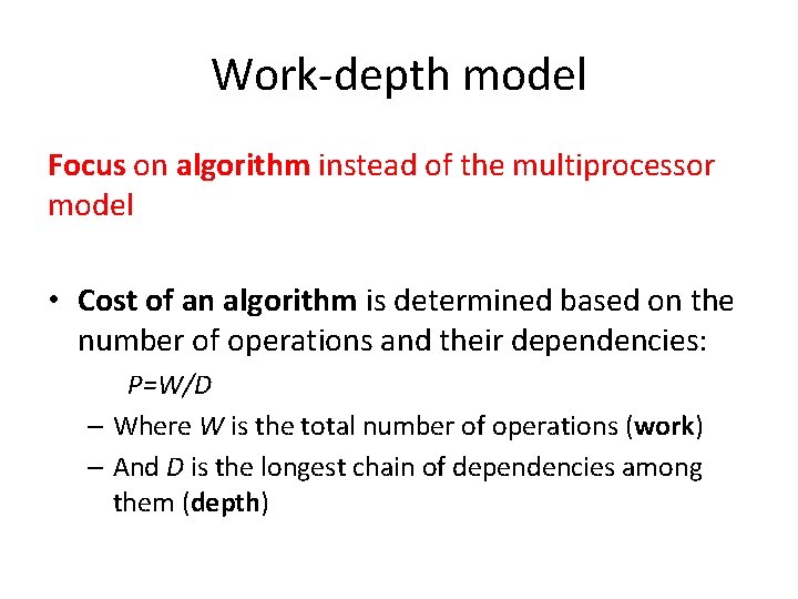
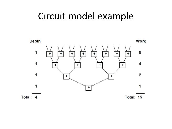
Work-depth model Focus on algorithm instead of the multiprocessor model • Cost of an algorithm is determined based on the number of operations and their dependencies: P=W/D – Where W is the total number of operations (work) – And D is the longest chain of dependencies among them (depth)

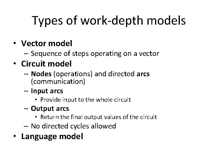
Types of work-depth models • Vector model – Sequence of steps operating on a vector • Circuit model – Nodes (operations) and directed arcs (communication) – Input arcs • Provide input to the whole circuit – Output arcs • Return the final output values of the circuit – No directed cycles allowed • Language model

Circuit model example

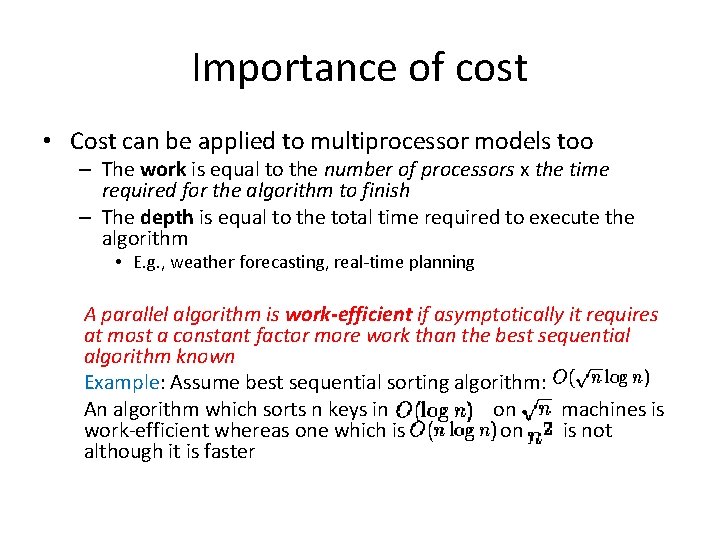
Importance of cost • Cost can be applied to multiprocessor models too – The work is equal to the number of processors x the time required for the algorithm to finish – The depth is equal to the total time required to execute the algorithm • E. g. , weather forecasting, real-time planning A parallel algorithm is work-efficient if asymptotically it requires at most a constant factor more work than the best sequential algorithm known Example: Assume best sequential sorting algorithm: An algorithm which sorts n keys in on machines is work-efficient whereas one which is on is not although it is faster

Takeaway slide Knowing Open. MP, MPI or Map. Reduce is good BUT • Writing parallel code is not enough! • We need to understand – Network topology – Hardware architecture, and – Data properties • • Data access patterns Structure of relational data (graphs – type? ) Location … Algorithm + Architecture + Data = Efficiency

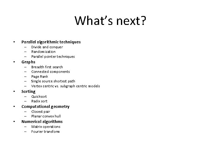
What’s next? • Parallel algorithmic techniques – – – • Graphs – – – • Quicksort Radix sort Computational geometry – – • Breadth first search Connected components Page Rank Single source shortest path Vertex centric vs. subgraph centric models Sorting – – • Divide and conquer Randomization Parallel pointer techniques Closest pair Planar convex hull Numerical algorithms – – Matrix operations Fourier transform

Evaluation • Presentation of a research article from a top journal or conference in the area of the lecture. • You will have to be able to – Understand the article – Present it to an audience – Discuss and propose future work