Parallel Algorithms Underlying MPI Implementations Parallel Algorithms Underlying

Parallel Algorithms Underlying MPI Implementations

Parallel Algorithms Underlying MPI Implementations • This chapter looks at a few of the parallel algorithms underlying the implementations of some simple MPI calls. • The purpose of this is not to teach you how to "roll your own" versions of these routines, but rather to help you start thinking about algorithms in a parallel fashion. • First, the method of recursive halving and doubling, which is the algorithm underlying operations such as broadcasts and reduction operations, is discussed. • Then, specific examples of parallel algorithms that implement message passing are given.

Recursive Halving and Doubling

Recursive Halving and Doubling • To illustrate recursive halving and doubling, suppose you have a vector distributed among p processors, and you need the sum of all components of the vector in each processor, i. e. , a sum reduction. • One method is to use a tree-based algorithm to compute the sum to a single processor and then broadcast the sum to every processor.

Recursive Halving and Doubling • Assume that each processor has formed the partial sum of the components of the vector that it has. • Step 1: Processor 2 sends its partial sum to processor 1 and processor 1 adds this partial sum to its own. Meanwhile, processor 4 sends its partial sum to processor 3 and processor 3 performs a similar summation. • Step 2: Processor 3 sends its partial sum, which is now the sum of the components on processors 3 and 4, to processor 1 and processor 1 adds it to its partial sum to get the final sum across all the components of the vector. • At each stage of the process, the number of processes doing work is cut in half. The algorithm is depicted in the Figure 13. 1 below, where the solid arrow denotes a send operation and the dotted line arrow denotes a receive operation followed by a summation.

Recursive Halving and Doubling Figure 13. 1. Summation in log(N) steps.

Recursive Halving and Doubling • Step 3: Processor 1 then must broadcast this sum to all other processors. This broadcast operation can be done using the same communication structure as the summation, but in reverse. You will see pseudocode for this at the end of this section. Note that if the total number of processors is N, then only 2 log(N) (log base 2) steps are needed to complete the operation. • There is an even more efficient way to finish the job in only log(N) steps. By way of example, look at the next figure containing 8 processors. At each step, processor i and processor i+k send and receive data in a pairwise fashion and then perform the summation. k is iterated from 1 through N/2 in powers of 2. If the total number of processors is N, then log(N) steps are needed. As an exercise, you should write out the necessary pseudocode for this example.

Recursive Halving and Doubling Figure 13. 2. Summation to all processors in log(N) steps.

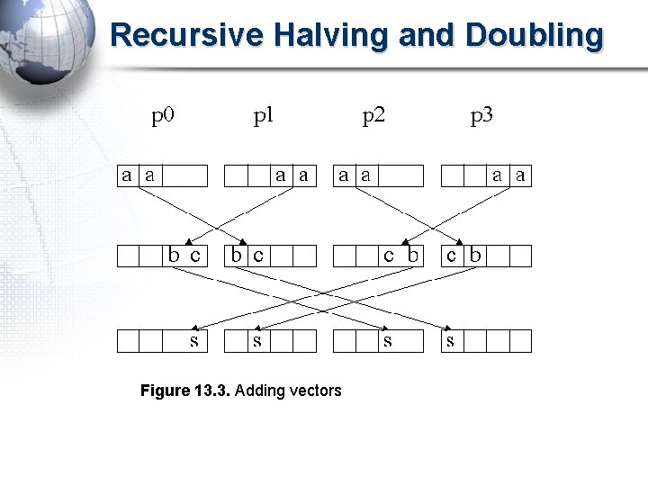
Recursive Halving and Doubling • What about adding vectors? That is, how do you add several vectors component-wise to get a new vector? The answer is, you employ the method discussed earlier in a component-wise fashion. This fascinating way to reduce the communications and to avoid abundant summations is described next. This method utilizes the recursive halving and doubling technique and is illustrated in Figure 13. 3.

Recursive Halving and Doubling • Suppose there are 4 processors and the length of each vector is also 4. • Step 1: Processor p 0 sends the first two components of the vector to processor p 1, and p 1 sends the last two components of the vector to p 0. Then p 0 gets the partial sums for the last two components, and p 1 gets the partial sums for the first two components. So do p 2 and p 3. • Step 2: Processor p 0 sends the partial sum of the third component to processor p 3. Processor p 3 then adds to get the total sum of the third component. Similarly, processor 0, 1 and 2 find the total sums of the 4 th, 2 nd, and 1 st components, respectively. Now the sum of the vectors are found and the components are stored in different processors. • Step 3: Broadcast the result using the reverse of the above communication process.

Recursive Halving and Doubling Figure 13. 3. Adding vectors

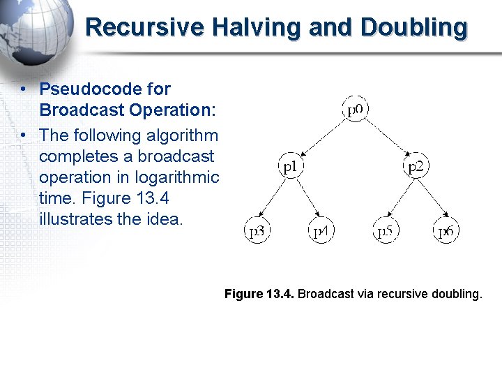
Recursive Halving and Doubling • Pseudocode for Broadcast Operation: • The following algorithm completes a broadcast operation in logarithmic time. Figure 13. 4 illustrates the idea. Figure 13. 4. Broadcast via recursive doubling.

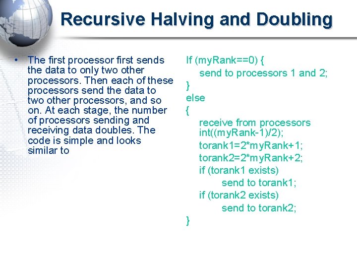
Recursive Halving and Doubling • The first processor first sends the data to only two other processors. Then each of these processors send the data to two other processors, and so on. At each stage, the number of processors sending and receiving data doubles. The code is simple and looks similar to If (my. Rank==0) { send to processors 1 and 2; } else { receive from processors int((my. Rank-1)/2); torank 1=2*my. Rank+1; torank 2=2*my. Rank+2; if (torank 1 exists) send to torank 1; if (torank 2 exists) send to torank 2; }

Parallel Algorithm Examples

Specific Examples • In this section, specific examples of parallel algorithms that implement message passing are given. • The first two examples consider simple collective communication calls to parallelize matrix-vector and matrix-matrix multiplication. • These calls are meant to be illustrative, because parallel numerical libraries usually provide the most efficient algorithms for these operations. (See Chapter 10 Parallel Mathematical Libraries. ) • The third example shows how you can use ghost cells to construct a parallel data approach to solve Poisson's equation. • The fourth example revisits matrix-vector multiplication, but from a client server approach.

Specific Examples • Example 1: – Matrix-vector multiplication using collective communication. • Example 2: – Matrix-matrix multiplication using collective communication. • Example 3: – Solving Poisson's equation through the use of ghost cells. • Example 4: – Matrix-vector multiplication using a client-server approach.

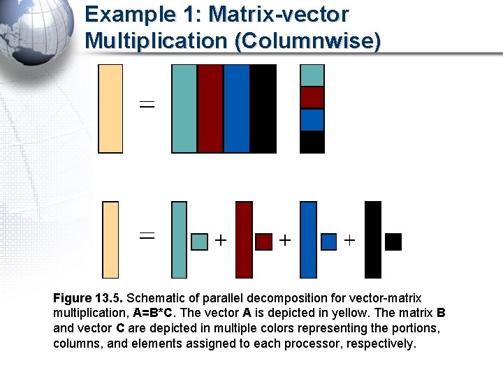
Example 1: Matrix-vector Multiplication • The figure below demonstrates schematically how a matrix-vector multiplication, A=B*C, can be decomposed into four independent computations involving a scalar multiplying a column vector. • This approach is different from that which is usually taught in a linear algebra course because this decomposition lends itself better to parallelization. • These computations are independent and do not require communication, something that usually reduces performance of parallel code.

Example 1: Matrix-vector Multiplication (Columnwise) Figure 13. 5. Schematic of parallel decomposition for vector-matrix multiplication, A=B*C. The vector A is depicted in yellow. The matrix B and vector C are depicted in multiple colors representing the portions, columns, and elements assigned to each processor, respectively.

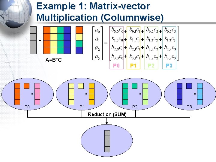
Example 1: Matrix-vector Multiplication (Columnwise) A=B*C P 0 + + + P 0 P 1 P 2 Reduction (SUM) P 2 P 3

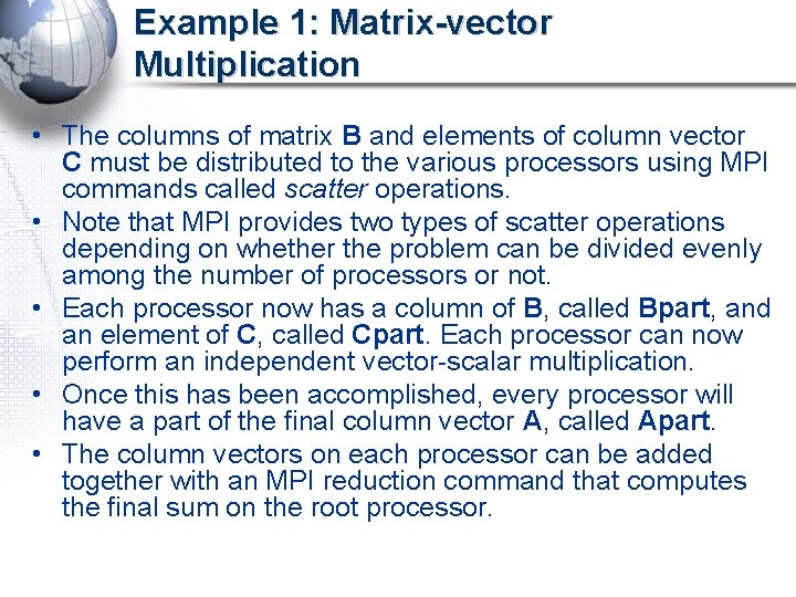
Example 1: Matrix-vector Multiplication • The columns of matrix B and elements of column vector C must be distributed to the various processors using MPI commands called scatter operations. • Note that MPI provides two types of scatter operations depending on whether the problem can be divided evenly among the number of processors or not. • Each processor now has a column of B, called Bpart, and an element of C, called Cpart. Each processor can now perform an independent vector-scalar multiplication. • Once this has been accomplished, every processor will have a part of the final column vector A, called Apart. • The column vectors on each processor can be added together with an MPI reduction command that computes the final sum on the root processor.

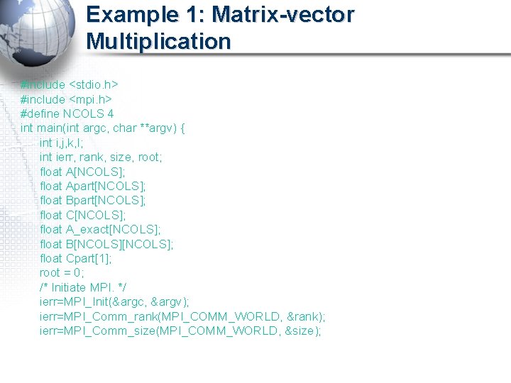
Example 1: Matrix-vector Multiplication #include <stdio. h> #include <mpi. h> #define NCOLS 4 int main(int argc, char **argv) { int i, j, k, l; int ierr, rank, size, root; float A[NCOLS]; float Apart[NCOLS]; float Bpart[NCOLS]; float C[NCOLS]; float A_exact[NCOLS]; float B[NCOLS]; float Cpart[1]; root = 0; /* Initiate MPI. */ ierr=MPI_Init(&argc, &argv); ierr=MPI_Comm_rank(MPI_COMM_WORLD, &rank); ierr=MPI_Comm_size(MPI_COMM_WORLD, &size);

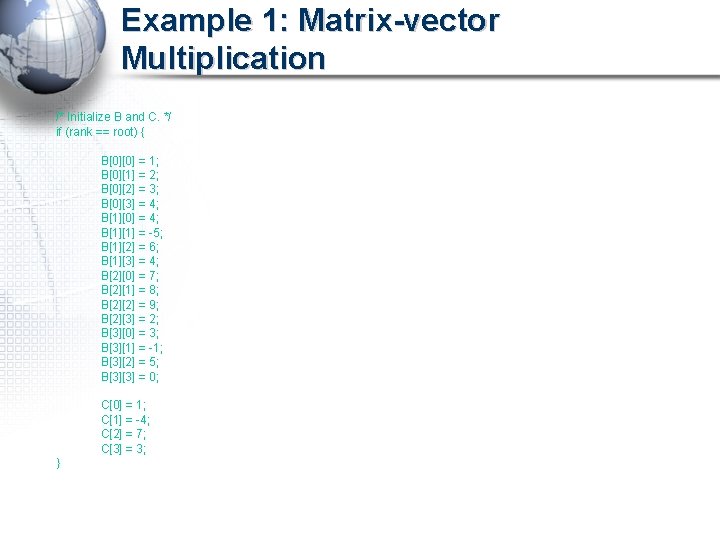
Example 1: Matrix-vector Multiplication /* Initialize B and C. */ if (rank == root) { B[0][0] = 1; B[0][1] = 2; B[0][2] = 3; B[0][3] = 4; B[1][0] = 4; B[1][1] = -5; B[1][2] = 6; B[1][3] = 4; B[2][0] = 7; B[2][1] = 8; B[2][2] = 9; B[2][3] = 2; B[3][0] = 3; B[3][1] = -1; B[3][2] = 5; B[3][3] = 0; C[0] = 1; C[1] = -4; C[2] = 7; C[3] = 3; }

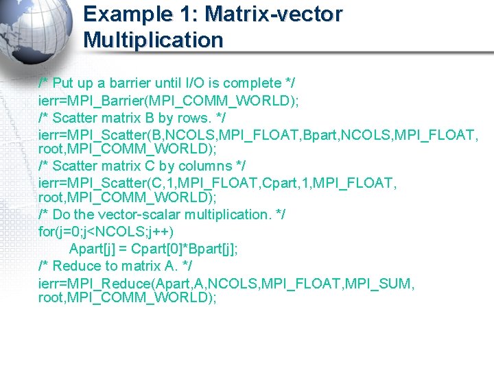
Example 1: Matrix-vector Multiplication /* Put up a barrier until I/O is complete */ ierr=MPI_Barrier(MPI_COMM_WORLD); /* Scatter matrix B by rows. */ ierr=MPI_Scatter(B, NCOLS, MPI_FLOAT, Bpart, NCOLS, MPI_FLOAT, root, MPI_COMM_WORLD); /* Scatter matrix C by columns */ ierr=MPI_Scatter(C, 1, MPI_FLOAT, Cpart, 1, MPI_FLOAT, root, MPI_COMM_WORLD); /* Do the vector-scalar multiplication. */ for(j=0; j<NCOLS; j++) Apart[j] = Cpart[0]*Bpart[j]; /* Reduce to matrix A. */ ierr=MPI_Reduce(Apart, A, NCOLS, MPI_FLOAT, MPI_SUM, root, MPI_COMM_WORLD);

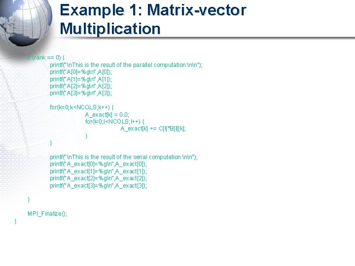
Example 1: Matrix-vector Multiplication if (rank == 0) { printf("n. This is the result of the parallel computation: nn"); printf("A[0]=%gn", A[0]); printf("A[1]=%gn", A[1]); printf("A[2]=%gn", A[2]); printf("A[3]=%gn", A[3]); for(k=0; k<NCOLS; k++) { A_exact[k] = 0. 0; for(l=0; l<NCOLS; l++) { A_exact[k] += C[l]*B[l][k]; } } printf("n. This is the result of the serial computation: nn"); printf("A_exact[0]=%gn", A_exact[0]); printf("A_exact[1]=%gn", A_exact[1]); printf("A_exact[2]=%gn", A_exact[2]); printf("A_exact[3]=%gn", A_exact[3]); } MPI_Finalize(); }

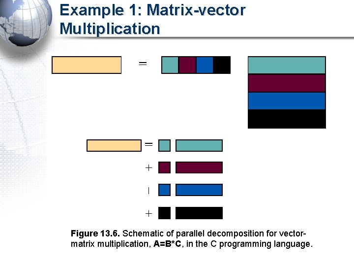
Example 1: Matrix-vector Multiplication • It is important to realize that this algorithm would change if the program were written in Fortran. This is because C decomposes arrays in memory by rows while Fortran decomposes arrays into columns. • If you translated the above program directly into a Fortran program, the collective MPI calls would fail because the data going to each of the different processors is not contiguous. • This problem can be solved with derived datatypes, which are discussed in Chapter 6 - Derived Datatypes. • A simpler approach would be to decompose the vectormatrix multiplication into independent scalar-row computations and then proceed as above. This approach is shown schematically in Figure 13. 6.

Example 1: Matrix-vector Multiplication Figure 13. 6. Schematic of parallel decomposition for vectormatrix multiplication, A=B*C, in the C programming language.

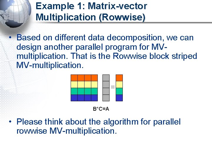
Example 1: Matrix-vector Multiplication (Rowwise) • Based on different data decomposition, we can design another parallel program for MVmultiplication. That is the Rowwise block striped MV-multiplication. B*C=A • Please think about the algorithm for parallel rowwise MV-multiplication.

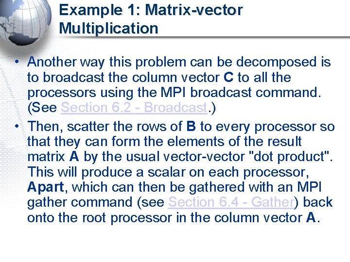
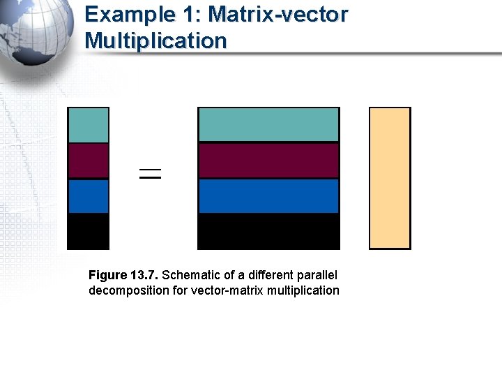
Example 1: Matrix-vector Multiplication • Another way this problem can be decomposed is to broadcast the column vector C to all the processors using the MPI broadcast command. (See Section 6. 2 - Broadcast. ) • Then, scatter the rows of B to every processor so that they can form the elements of the result matrix A by the usual vector-vector "dot product". This will produce a scalar on each processor, Apart, which can then be gathered with an MPI gather command (see Section 6. 4 - Gather) back onto the root processor in the column vector A.

Example 1: Matrix-vector Multiplication Figure 13. 7. Schematic of a different parallel decomposition for vector-matrix multiplication

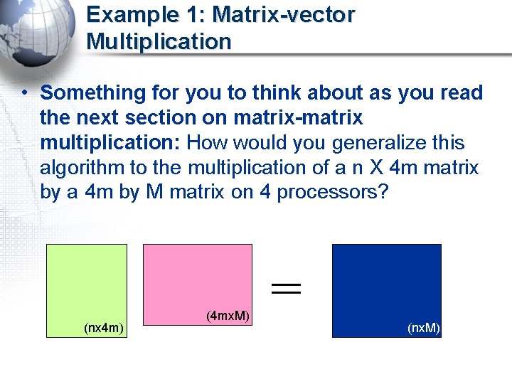
Example 1: Matrix-vector Multiplication • Something for you to think about as you read the next section on matrix-matrix multiplication: How would you generalize this algorithm to the multiplication of a n X 4 m matrix by a 4 m by M matrix on 4 processors? (nx 4 m) (4 mx. M) (nx. M)

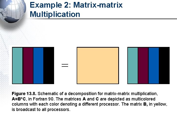
Example 2: Matrix-matrix Multiplication • A similar, albeit naive, type of decomposition can be achieved for matrix-matrix multiplication, A=B*C. • The figure below shows schematically how matrix -matrix multiplication of two 4 x 4 matrices can be decomposed into four independent vector-matrix multiplications, which can be performed on four different processors.

Example 2: Matrix-matrix Multiplication Figure 13. 8. Schematic of a decomposition for matrix-matrix multiplication, A=B*C, in Fortran 90. The matrices A and C are depicted as multicolored columns with each color denoting a different processor. The matrix B, in yellow, is broadcast to all processors.

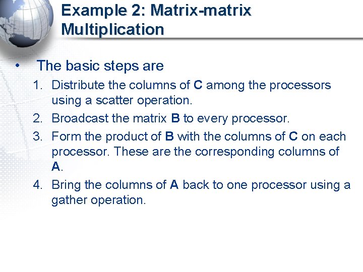
Example 2: Matrix-matrix Multiplication • The basic steps are 1. Distribute the columns of C among the processors using a scatter operation. 2. Broadcast the matrix B to every processor. 3. Form the product of B with the columns of C on each processor. These are the corresponding columns of A. 4. Bring the columns of A back to one processor using a gather operation.

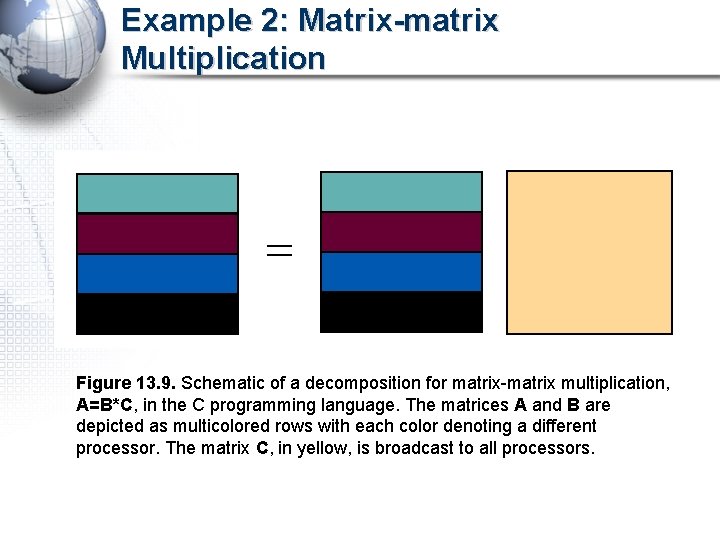
Example 2: Matrix-matrix Multiplication • Again, in C, the problem could be decomposed in rows. This is shown schematically below. • The code is left as your homework!!!

Example 2: Matrix-matrix Multiplication Figure 13. 9. Schematic of a decomposition for matrix-matrix multiplication, A=B*C, in the C programming language. The matrices A and B are depicted as multicolored rows with each color denoting a different processor. The matrix C, in yellow, is broadcast to all processors.

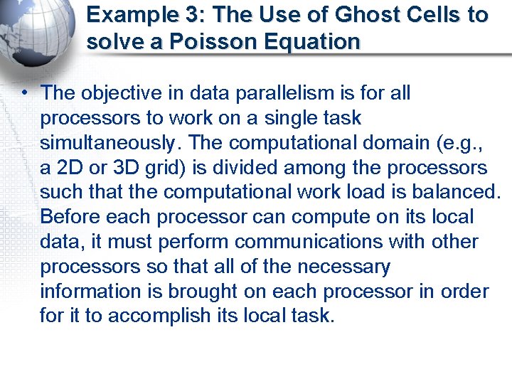
Example 3: The Use of Ghost Cells to solve a Poisson Equation • The objective in data parallelism is for all processors to work on a single task simultaneously. The computational domain (e. g. , a 2 D or 3 D grid) is divided among the processors such that the computational work load is balanced. Before each processor can compute on its local data, it must perform communications with other processors so that all of the necessary information is brought on each processor in order for it to accomplish its local task.

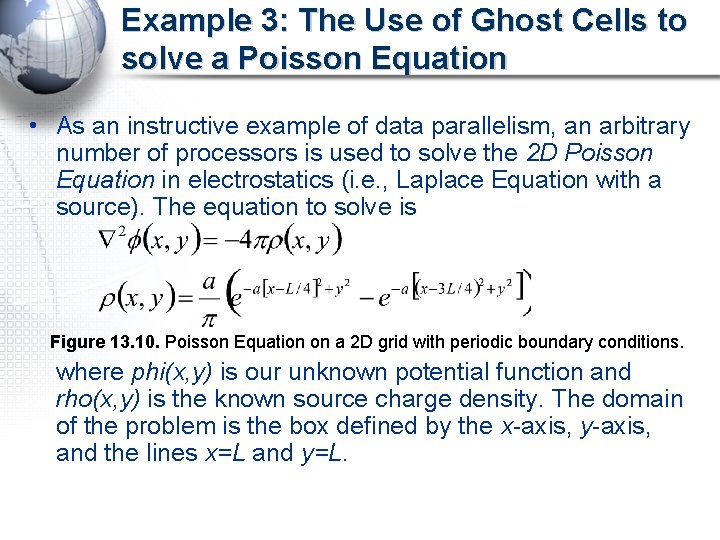
Example 3: The Use of Ghost Cells to solve a Poisson Equation • As an instructive example of data parallelism, an arbitrary number of processors is used to solve the 2 D Poisson Equation in electrostatics (i. e. , Laplace Equation with a source). The equation to solve is Figure 13. 10. Poisson Equation on a 2 D grid with periodic boundary conditions. where phi(x, y) is our unknown potential function and rho(x, y) is the known source charge density. The domain of the problem is the box defined by the x-axis, y-axis, and the lines x=L and y=L.

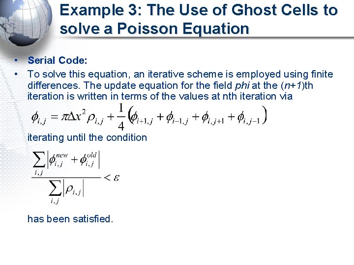
Example 3: The Use of Ghost Cells to solve a Poisson Equation • Serial Code: • To solve this equation, an iterative scheme is employed using finite differences. The update equation for the field phi at the (n+1)th iteration is written in terms of the values at nth iteration via iterating until the condition has been satisfied.

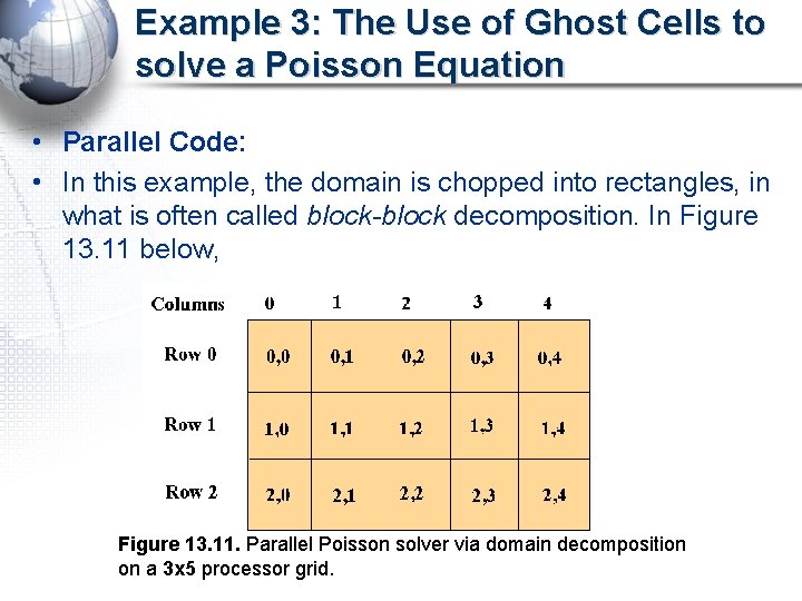
Example 3: The Use of Ghost Cells to solve a Poisson Equation • Parallel Code: • In this example, the domain is chopped into rectangles, in what is often called block-block decomposition. In Figure 13. 11 below, Figure 13. 11. Parallel Poisson solver via domain decomposition on a 3 x 5 processor grid.

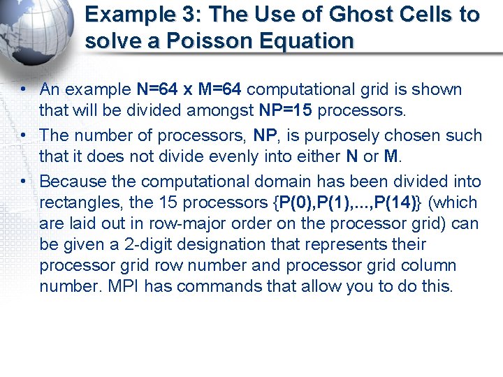
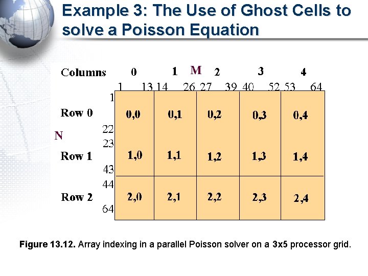
Example 3: The Use of Ghost Cells to solve a Poisson Equation • An example N=64 x M=64 computational grid is shown that will be divided amongst NP=15 processors. • The number of processors, NP, is purposely chosen such that it does not divide evenly into either N or M. • Because the computational domain has been divided into rectangles, the 15 processors {P(0), P(1), . . . , P(14)} (which are laid out in row-major order on the processor grid) can be given a 2 -digit designation that represents their processor grid row number and processor grid column number. MPI has commands that allow you to do this.

Example 3: The Use of Ghost Cells to solve a Poisson Equation Figure 13. 12. Array indexing in a parallel Poisson solver on a 3 x 5 processor grid.

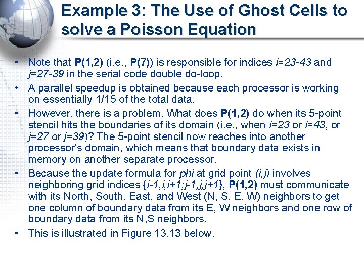
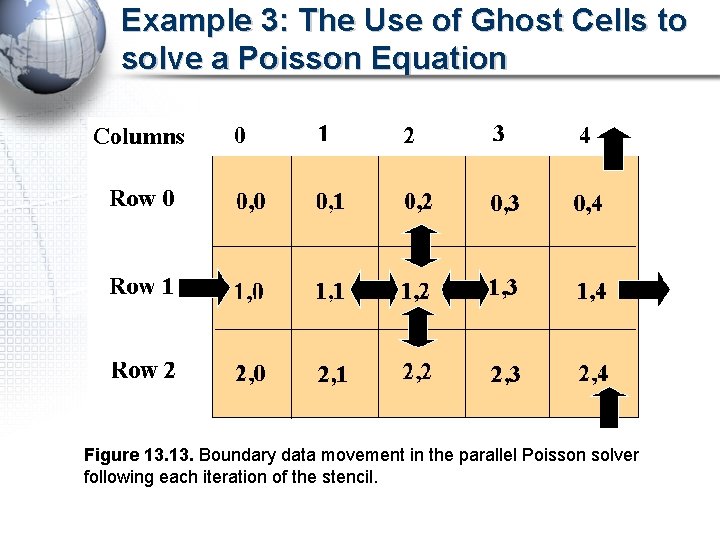
Example 3: The Use of Ghost Cells to solve a Poisson Equation • Note that P(1, 2) (i. e. , P(7)) is responsible for indices i=23 -43 and j=27 -39 in the serial code double do-loop. • A parallel speedup is obtained because each processor is working on essentially 1/15 of the total data. • However, there is a problem. What does P(1, 2) do when its 5 -point stencil hits the boundaries of its domain (i. e. , when i=23 or i=43, or j=27 or j=39)? The 5 -point stencil now reaches into another processor's domain, which means that boundary data exists in memory on another separate processor. • Because the update formula for phi at grid point (i, j) involves neighboring grid indices {i-1, i, i+1; j-1, j, j+1}, P(1, 2) must communicate with its North, South, East, and West (N, S, E, W) neighbors to get one column of boundary data from its E, W neighbors and one row of boundary data from its N, S neighbors. • This is illustrated in Figure 13. 13 below.

Example 3: The Use of Ghost Cells to solve a Poisson Equation Figure 13. Boundary data movement in the parallel Poisson solver following each iteration of the stencil.

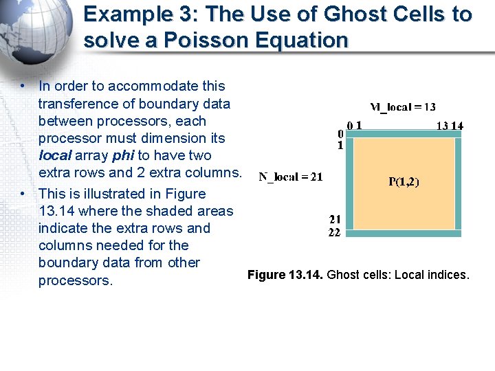
Example 3: The Use of Ghost Cells to solve a Poisson Equation • In order to accommodate this transference of boundary data between processors, each processor must dimension its local array phi to have two extra rows and 2 extra columns. • This is illustrated in Figure 13. 14 where the shaded areas indicate the extra rows and columns needed for the boundary data from other Figure 13. 14. Ghost cells: Local indices. processors.

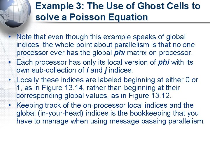
Example 3: The Use of Ghost Cells to solve a Poisson Equation • Note that even though this example speaks of global indices, the whole point about parallelism is that no one processor ever has the global phi matrix on processor. • Each processor has only its local version of phi with its own sub-collection of i and j indices. • Locally these indices are labeled beginning at either 0 or 1, as in Figure 13. 14, rather than beginning at their corresponding global values, as in Figure 13. 12. • Keeping track of the on-processor local indices and the global (in-your-head) indices is the bookkeeping that you have to manage when using message passing parallelism.

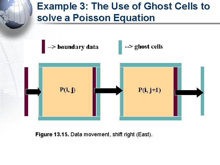
Example 3: The Use of Ghost Cells to solve a Poisson Equation • Other parallel paradigms, such as High Performance Fortran (HPF) or Open. MP, are directive-based, i. e. , compiler directives are inserted into the code to tell the supercomputer to distribute data across processors or to perform other operations. The difference between the two paradigms is akin to the difference between an automatic and stick-shift transmission car. • In the directive based paradigm (automatic), the compiler (car) does the data layout and parallel communications (gear shifting) implicitly. • In the message passing paradigm (stick-shift), the user (driver) performs the data layout and parallel communications explicitly. In this example, this communication can be performed in a regular prescribed pattern for all processors. • For example, all processors could first communicate with their Nmost partners, then S, then E, then W. What is happening when all processors communicate with their E neighbors is illustrated in Figure 13. 15.

Example 3: The Use of Ghost Cells to solve a Poisson Equation Figure 13. 15. Data movement, shift right (East).

Example 3: The Use of Ghost Cells to solve a Poisson Equation • • Note that in this shift right communication, P(i, j) places its right-most column of boundary data into the left-most ghost column of P(i, j+1). In addition, P(i, j) receives the right-most column of boundary data from P(i, j-1) into its own left-most ghost column. For each iteration, the psuedo-code for the parallel algorithm is thus t=0 (0) Initialize psi (1) Loop over stencil iterations (2) (3) (4) (5) (6) Perform parallel N shift communications of boundary data Perform parallel S shift communications of boundary data Perform parallel E shift communications of boundary data Perform parallel W shift communications of boundary data for{i=1; i<=N_local; i++){ for(j=1; j<=M_local; j++){ update phi[i][j] } } End Loop over stencil iterations (7) Output data

Example 3: The Use of Ghost Cells to solve a Poisson Equation • Note that initializing the data should be performed in parallel. That is, each processor P(i, j) should only initialize the portion of phi for which it is responsible. (Recall NO processor contains the full global phi). • In relation to this point, step (7), Output data, is not such a simpleminded task when performing parallel calculations. Should you reduce all the data from phi_local on each processor to one giant phi_global on P(0, 0) and then print out the data? This is certainly one way to do it, but it seems to defeat the purpose of not having all the data reside on one processor. • For example, what if phi_global is too large to fit in memory on a single processor? A second alternative is for each processor to write out its own phi_local to a file "phi. ij", where ij indicates the processor's 2 -digit designation (e. g. P(1, 2) writes out to file "phi. 12"). • The data then has to be manipulated off processor by another code to put it into a form that may be rendered by a visualization package. This code itself may have to be a parallel code.

Example 3: The Use of Ghost Cells to solve a Poisson Equation • As you can see, the issue of parallel I/O is not a trivial one (see Section 9 - Parallel I/O) and is in fact a topic of current research among parallel language developers and researchers.

Matrix-vector Multiplication using a Client-Server Approach • • In Section 13. 2. 1, a simple data decomposition for multiplying a matrix and a vector was described. This decomposition is also used here to demonstrate a "client-server" approach. The code for this example is in the C program, server_client_c. c. In server_client_c. c, all input/output is handled by the "server" (preset to be processor 0). This includes parsing the command-line arguments, reading the file containing the matrix A and vector x, and writing the result to standard output. The file containing the matrix A and the vector x has the form m x 1 a 11 a 21. . . n x 2. . . a 12. . . a 22. . . where A is m (rows) by n (columns), and x is a column vector with n elements.

Matrix-vector Multiplication using a Client-Server Approach • After the server reads in the size of A, it broadcasts this information to all of the clients. • It then checks to make sure that there are fewer processors than columns. (If there are more processors than columns, then using a parallel program is not efficient and the program exits. ) • The server and all of the clients then allocate memory locations for A and x. The server also allocates memory for the result. • Because there are more columns than client processors, the first "round" consists of the server sending one column to each of the client processors. • All of the clients receive a column to process. Upon finishing, the clients send results back to the server. As the server receives a "result" buffer from a client, it sends the next unprocessed column to that client.

Matrix-vector Multiplication using a Client-Server Approach • The source code is divided into two sections: the "server" code and the "client" code. The pseudo-code for each of these sections is • Server: – Broadcast (vector) x to all client processors. – Send a column of A to each processor. – While there are more columns to process OR there are expected results, receive results and send next unprocessed column. – Print result. • Client: – Receive (vector) x. – Receive a column of A with tag = column number. – Multiply respective element of (vector) x (which is the same as tag) to produce the (vector) result. – Send result back to server. • Note that the numbers used in the pseudo-code (for both the server and client) have been added to the source code.

Matrix-vector Multiplication using a Client-Server Approach • Source code similar to server_client_c. c. , server_client_r. c is also provided as an example. • The main difference between theses codes is the way the data is stored. • Because only contiguous memory locations can be sent using MPI_SEND, server_client_c. c stores the matrix A "column-wise" in memory, while server_client_r. c stores the matrix A "row-wise" in memory. • The pseudo-code for server_client_c. c and server_client_r. c is stated in the "block" documentation at the beginning of the source code.

END