Data Structures Algorithms Lecture 1 Data Structures Algorithms

Data Structures & Algorithms Lecture # 1

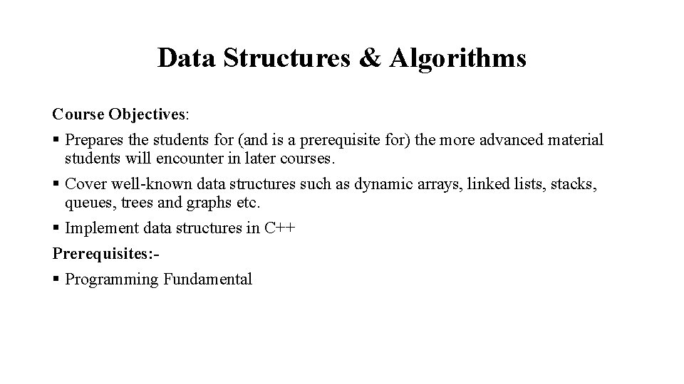
Data Structures & Algorithms Course Objectives: § Prepares the students for (and is a prerequisite for) the more advanced material students will encounter in later courses. § Cover well-known data structures such as dynamic arrays, linked lists, stacks, queues, trees and graphs etc. § Implement data structures in C++ Prerequisites: § Programming Fundamental

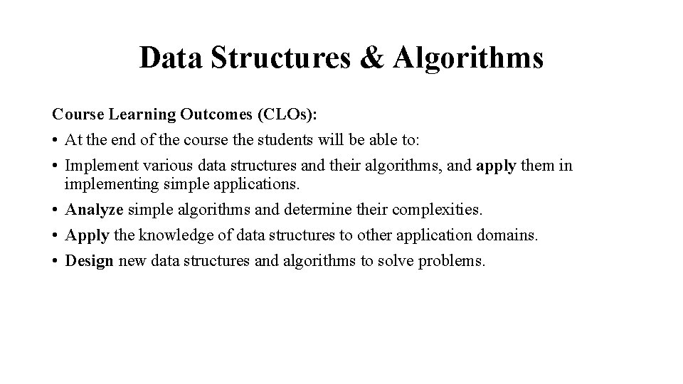
Data Structures & Algorithms Course Learning Outcomes (CLOs): • At the end of the course the students will be able to: • Implement various data structures and their algorithms, and apply them in implementing simple applications. • Analyze simple algorithms and determine their complexities. • Apply the knowledge of data structures to other application domains. • Design new data structures and algorithms to solve problems.

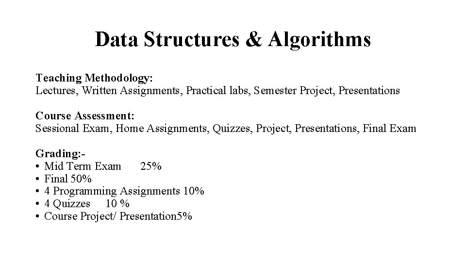
Data Structures & Algorithms Teaching Methodology: Lectures, Written Assignments, Practical labs, Semester Project, Presentations Course Assessment: Sessional Exam, Home Assignments, Quizzes, Project, Presentations, Final Exam Grading: • Mid Term Exam 25% • Final 50% • 4 Programming Assignments 10% • 4 Quizzes 10 % • Course Project/ Presentation 5%

Data Structures & Algorithms Course Content: Introduction to Data Structures and Algorithms; Abstract data types, complexity analysis, Big Oh notation, Stacks (linked lists and array implementations), Recursion and analyzing recursive algorithms, divide and conquer algorithms, Sorting algorithms (selection, insertion, merge, quick, bubble, heap, shell, radix, bucket), queue, dequeuer, priority queues (linked and array implementations of queues), linked list & its various types, sorted linked list, searching an unsorted array, binary search for sorted arrays, hashing and indexing, open addressing and chaining, trees and tree traversals, binary search trees, heaps, M-way tress, balanced trees, graphs, breadth-first and depth-first traversal, topological order, shortest path, adjacency matrix and adjacency list implementations, memory management and garbage collection.

Data Structures & Algorithms Recommended Readings: 1. Data Structures and Algorithms in C++ by Adam Drozdek 2. Data Structures and Algorithm Analysis in Java by Mark A. Weiss 3. Data Structures and Abstractions with Java by Frank M. Carrano & Timothy M. Henry 4. Data Structures and Algorithm Analysis in C++ by Mark Allen Weiss 5. Java Software Structures: Designing and Using Data Structures by John Lewis and Joseph Chase.

Data Structures & Algorithms Need for Data Structures: • Data structures organize data more efficient programs. • More powerful computers more complex applications. • More complex applications demand more calculations. • Data Structure means any organization of data, that can be searched, processed in any order, or modified. • The choice of data structure and algorithm can make the difference between a program running in a few seconds or many days.

Data Structures & Algorithms Efficiency: § A solution is said to be efficient if it solves the problem within its resource constraints. • Space • Time § The cost of a solution is the amount of resources that the solution consumes.

Data Structures & Algorithms Select a data structure as follows: § Analyze the problem to determine the resource constraints a solution must meet. § Determine the basic operations that must be supported. Quantify the resource constraints for each operation. § Select the data structure that best meets these requirements. Some Questions to Ask? § Are all data inserted into the data structure at the beginning, or insertions interspersed with other operations? § Can data be deleted? § Are all data processed in some well-defined order, or is random access allowed?

Data Structures & Algorithms § Each data structure has costs and benefits. § Rarely is one data structure better than another in all situations. § A data structure requires: • space for each data item it stores, • time to perform each basic operation, • programming effort.

Data Structures & Algorithms History of Algorithm: The word algorithm comes from the name of the 9 th century Persian mathematician Abu Ja, far Muhammad ibn Musa al-Khwarzimi. He worked in Baghdad at the time when it was the center of scientific studies and trade. Al-Khwarzimi's name was translated into Latin, and eventually became algorithm. Algorithm: An algorithm is any well-define computational procedure that take some values or set of values as input and produce some values or set of values as output. OR A clearly specified set of simple instructions to be followed to solve a problem.

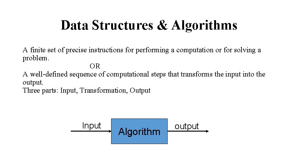
Data Structures & Algorithms A finite set of precise instructions for performing a computation or for solving a problem. OR A well-defined sequence of computational steps that transforms the input into the output. Three parts: Input, Transformation, Output Input Algorithm output

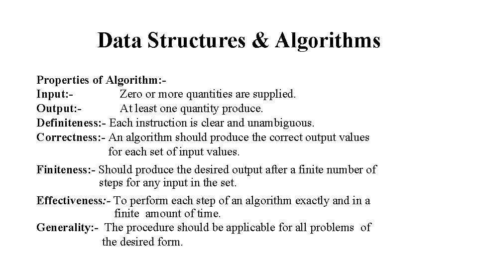
Data Structures & Algorithms Properties of Algorithm: Input: Zero or more quantities are supplied. Output: At least one quantity produce. Definiteness: - Each instruction is clear and unambiguous. Correctness: - An algorithm should produce the correct output values for each set of input values. Finiteness: - Should produce the desired output after a finite number of steps for any input in the set. Effectiveness: - To perform each step of an algorithm exactly and in a finite amount of time. Generality: - The procedure should be applicable for all problems of the desired form.

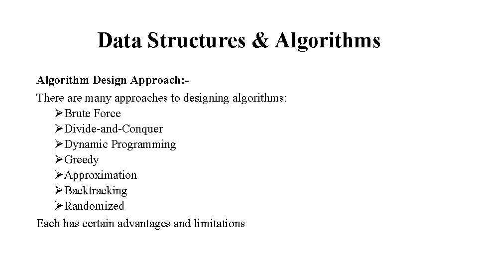
Data Structures & Algorithms Algorithm Design Approach: There are many approaches to designing algorithms: ØBrute Force ØDivide-and-Conquer ØDynamic Programming ØGreedy ØApproximation ØBacktracking ØRandomized Each has certain advantages and limitations

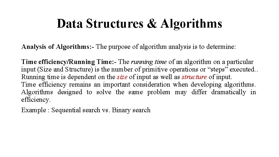
Data Structures & Algorithms Analysis of Algorithms: - The purpose of algorithm analysis is to determine: Time efficiency/Running Time: - The running time of an algorithm on a particular input (Size and Structure) is the number of primitive operations or “steps” executed. . Running time is dependent on the size of input as well as structure of input. Time efficiency remains an important consideration when developing algorithms. Algorithms designed to solve the same problem may differ dramatically in efficiency. Example : Sequential search vs. Binary search

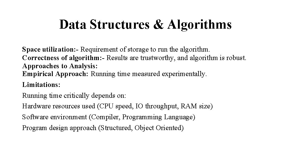
Data Structures & Algorithms Space utilization: - Requirement of storage to run the algorithm. Correctness of algorithm: - Results are trustworthy, and algorithm is robust. Approaches to Analysis: Empirical Approach: Running time measured experimentally. Limitations: Running time critically depends on: Hardware resources used (CPU speed, IO throughput, RAM size) Software environment (Compiler, Programming Language) Program design approach (Structured, Object Oriented)

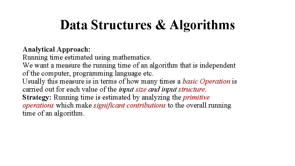
Data Structures & Algorithms Analytical Approach: Running time estimated using mathematics. We want a measure the running time of an algorithm that is independent of the computer, programming language etc. Usually this measure is in terms of how many times a basic Operation is carried out for each value of the input size and input structure. Strategy: Running time is estimated by analyzing the primitive operations which make significant contributions to the overall running time of an algorithm.

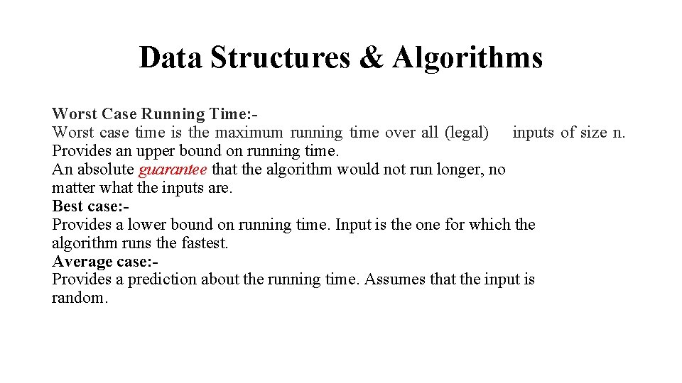
Data Structures & Algorithms Worst Case Running Time: Worst case time is the maximum running time over all (legal) inputs of size n. Provides an upper bound on running time. An absolute guarantee that the algorithm would not run longer, no matter what the inputs are. Best case: Provides a lower bound on running time. Input is the one for which the algorithm runs the fastest. Average case: Provides a prediction about the running time. Assumes that the input is random.

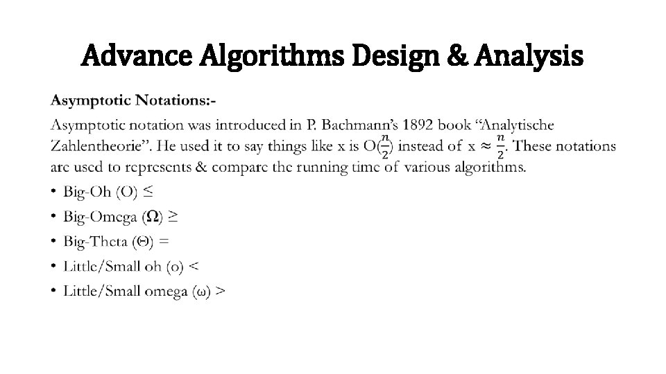
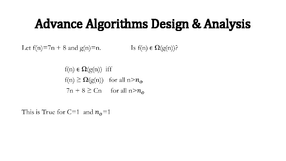
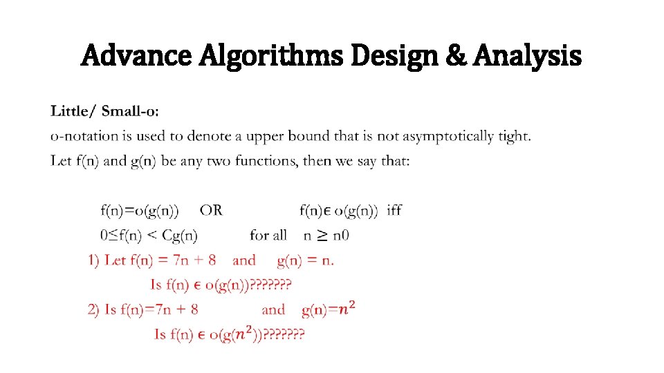
Advance Algorithms Design & Analysis •

Advance Algorithms Design & Analysis •

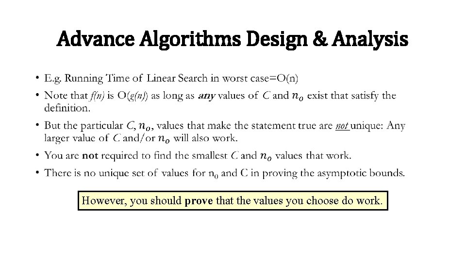
Advance Algorithms Design & Analysis • However, you should prove that the values you choose do work.

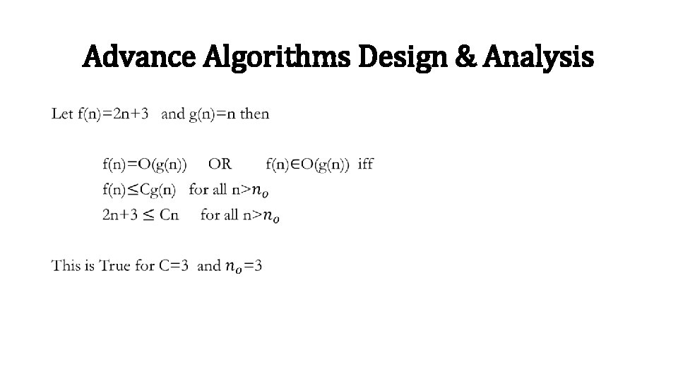
Advance Algorithms Design & Analysis •

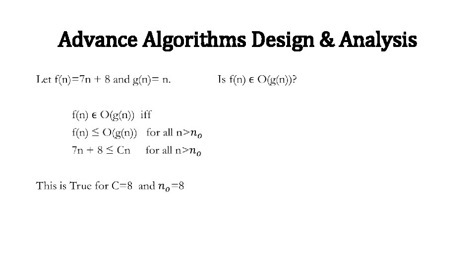
Advance Algorithms Design & Analysis •

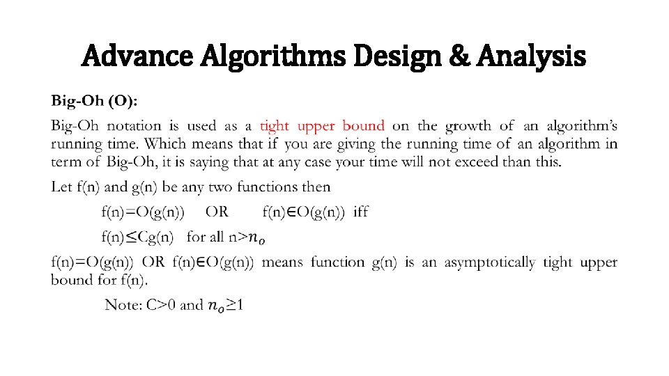
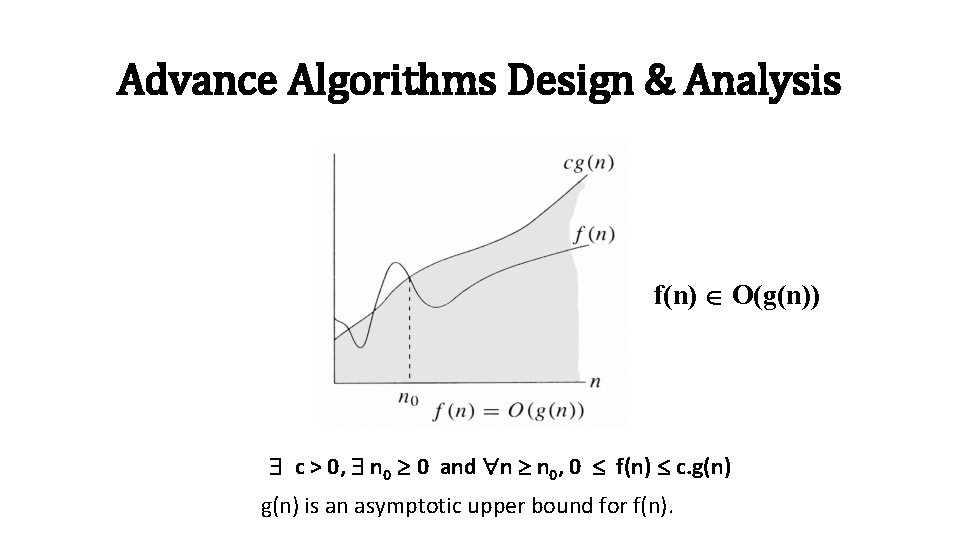
Advance Algorithms Design & Analysis f(n) O(g(n)) c > 0, n 0 0 and n n 0, 0 f(n) c. g(n) is an asymptotic upper bound for f(n).

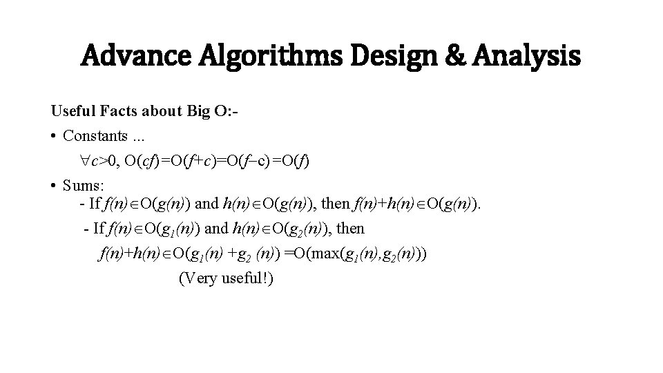
Advance Algorithms Design & Analysis Useful Facts about Big O: • Constants. . . c>0, O(cf)=O(f+c)=O(f) • Sums: - If f(n) O(g(n)) and h(n) O(g(n)), then f(n)+h(n) O(g(n)). - If f(n) O(g 1(n)) and h(n) O(g 2(n)), then f(n)+h(n) O(g 1(n) +g 2 (n)) =O(max(g 1(n), g 2(n))) (Very useful!)

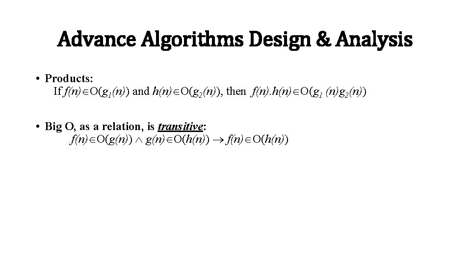
Advance Algorithms Design & Analysis • Products: If f(n) O(g 1(n)) and h(n) O(g 2(n)), then f(n). h(n) O(g 1 (n)g 2(n)) • Big O, as a relation, is transitive: f(n) O(g(n)) g(n) O(h(n)) f(n) O(h(n))

Advance Algorithms Design & Analysis •

Advance Algorithms Design & Analysis •

Advance Algorithms Design & Analysis •

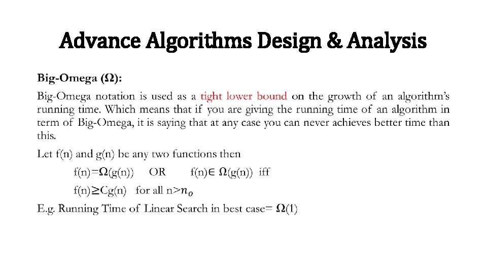
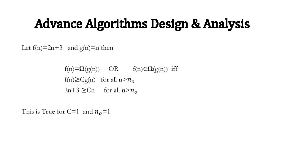
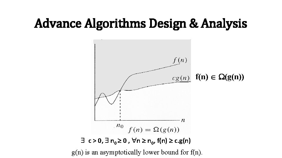
Advance Algorithms Design & Analysis f(n) (g(n)) c > 0, n 0 0 , n n 0, f(n) c. g(n) is an asymptotically lower bound for f(n).

Advance Algorithms Design & Analysis •

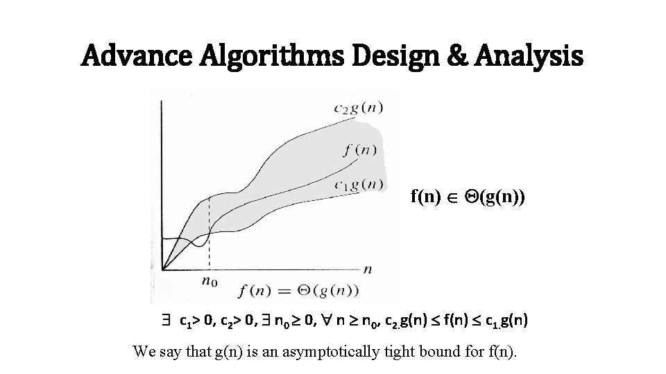
Advance Algorithms Design & Analysis f(n) (g(n)) c 1> 0, c 2> 0, n 0 0, n n 0, c 2. g(n) f(n) c 1. g(n) We say that g(n) is an asymptotically tight bound for f(n).

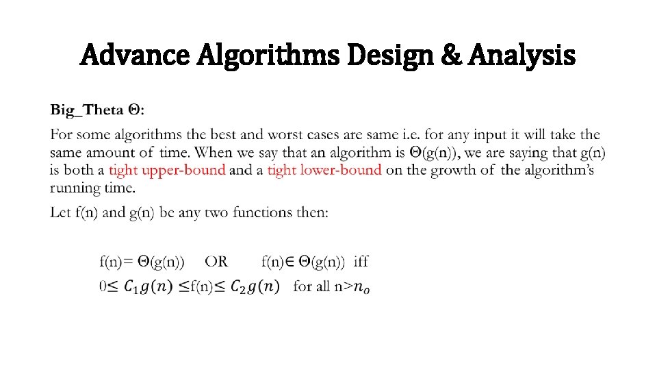
Advance Algorithms Design & Analysis •

Advance Algorithms Design & Analysis •

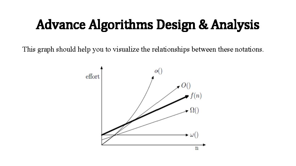
Advance Algorithms Design & Analysis This graph should help you to visualize the relationships between these notations.

Data Structures & Algorithms Array: Elementary data structure that exists as built-in in most programming languages. main( ) { int x[6]; int j; for(j=0; j < 6; j++) x[j] = 2*j; }

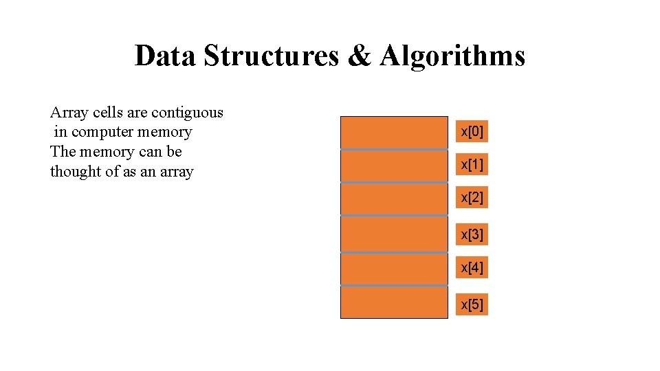
Data Structures & Algorithms § § § Array declaration: int x[6]; An array is collection of consecutive memory cells of the same name and type. The collection has the name ‘x’. The cells are numbered with consecutive integers. To access a cell, use the array name and an index: x[0], x[1], x[2], x[3], x[4], x[5]

Data Structures & Algorithms Array cells are contiguous in computer memory The memory can be thought of as an array x[0] x[1] x[2] x[3] x[4] x[5]

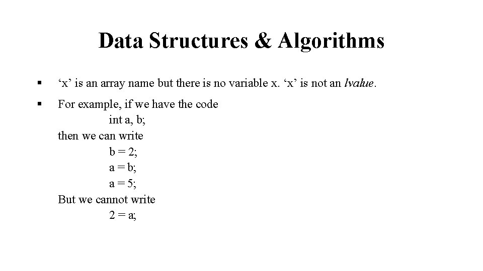
Data Structures & Algorithms § ‘x’ is an array name but there is no variable x. ‘x’ is not an lvalue. § For example, if we have the code int a, b; then we can write b = 2; a = b; a = 5; But we cannot write 2 = a;

Data Structures & Algorithms § ‘x’ is not an lvalue int x[6]; int n; x[0] = 5; x[1] = 2; x = 3; x = a + b; x = &n; // not allowed

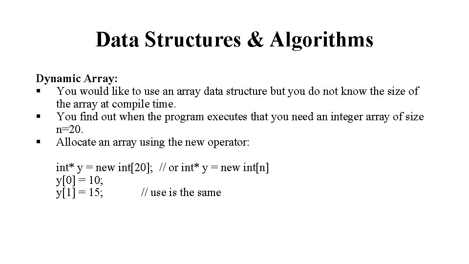
Data Structures & Algorithms Dynamic Array: § You would like to use an array data structure but you do not know the size of the array at compile time. § You find out when the program executes that you need an integer array of size n=20. § Allocate an array using the new operator: int* y = new int[20]; // or int* y = new int[n] y[0] = 10; y[1] = 15; // use is the same

Data Structures & Algorithms § § § ‘y’ is a lvalue; it is a pointer that holds the address of 20 consecutive cells in memory. It can be assigned a value. The new operator returns as address that is stored in y. We can write: y = &x[0]; y = x; // x can appear on the right // y gets the address of the // first cell of the x array

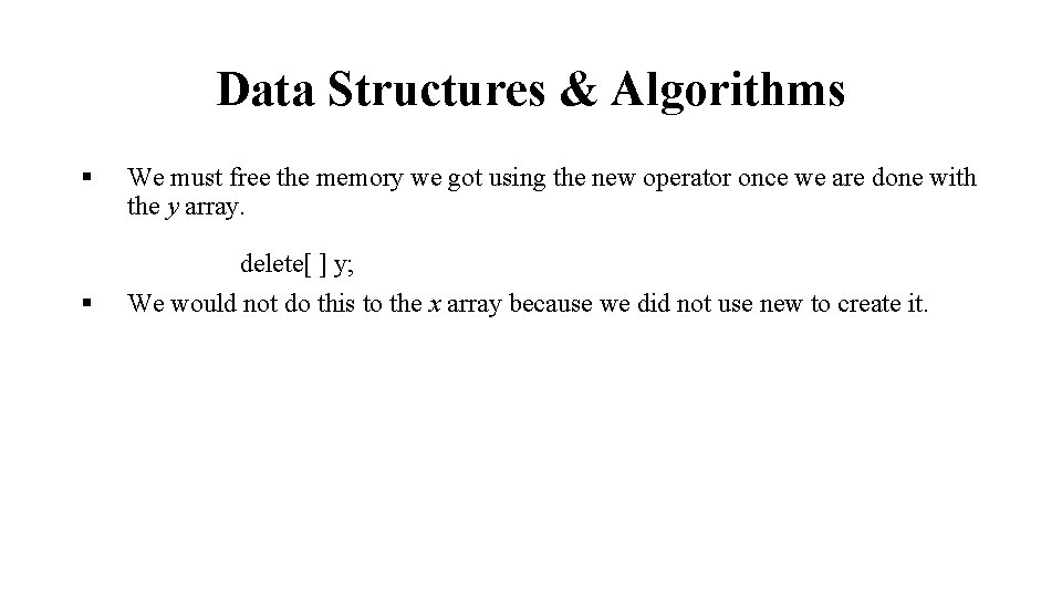
Data Structures & Algorithms § § We must free the memory we got using the new operator once we are done with the y array. delete[ ] y; We would not do this to the x array because we did not use new to create it.

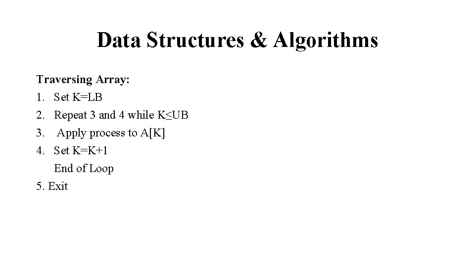
Data Structures & Algorithms Traversing Array: 1. Set K=LB 2. Repeat 3 and 4 while K≤UB 3. Apply process to A[K] 4. Set K=K+1 End of Loop 5. Exit

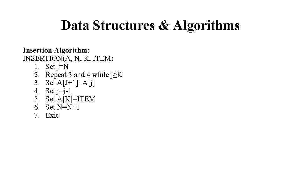
Data Structures & Algorithms Insertion Algorithm: INSERTION(A, N, K, ITEM) 1. Set j=N 2. Repeat 3 and 4 while j≥K 3. Set A[J+1]=A[j] 4. Set j=j-1 5. Set A[K]=ITEM 6. Set N=N+1 7. Exit

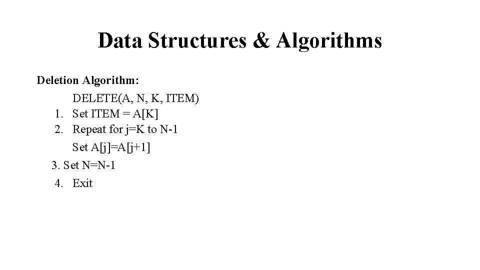
Data Structures & Algorithms Deletion Algorithm: DELETE(A, N, K, ITEM) 1. Set ITEM = A[K] 2. Repeat for j=K to N-1 Set A[j]=A[j+1] 3. Set N=N-1 4. Exit

Data Structures & Algorithms Searching: The operation to find the location of particular data item in list; There are two methods to find the location of data item in the array 1) Linear Search 2) Binary Search Linear Search: The simplest and direct approach, scan the entire list, one record at a time, for a given value. If found return the location otherwise the search is not successful.

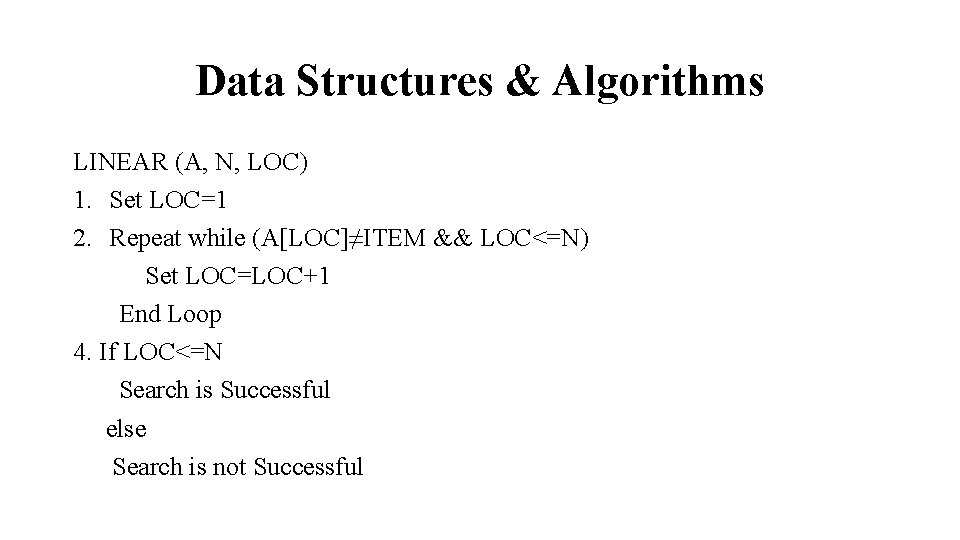
Data Structures & Algorithms LINEAR (A, N, LOC) 1. Set LOC=1 2. Repeat while (A[LOC]≠ITEM && LOC<=N) Set LOC=LOC+1 End Loop 4. If LOC<=N Search is Successful else Search is not Successful

Data Structures & Algorithms BINARY(A, LB, UB, ITEM LOC) 1. Set BEG=LB, END =UB , MID= (LB+UB)/2 2. Repeat 3 and 4 while BEG≤END and A[MID]≠ITEM 3. If ITEM<A[MID] Set END=MID-1 Else Set BEG=MID+1 4. Set MID=INT(BEG+END)/2 5. If A[MID]=ITEM LOC=MID Else LOC=NULL

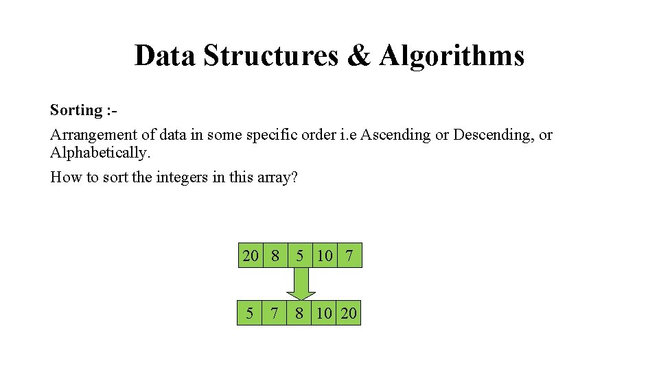
Data Structures & Algorithms Sorting : Arrangement of data in some specific order i. e Ascending or Descending, or Alphabetically. How to sort the integers in this array? 20 8 5 10 7 5 8 10 20 7

Data Structures & Algorithms Elementary Sorting Algorithms: • Selection Sort • Insertion Sort • Bubble Sort

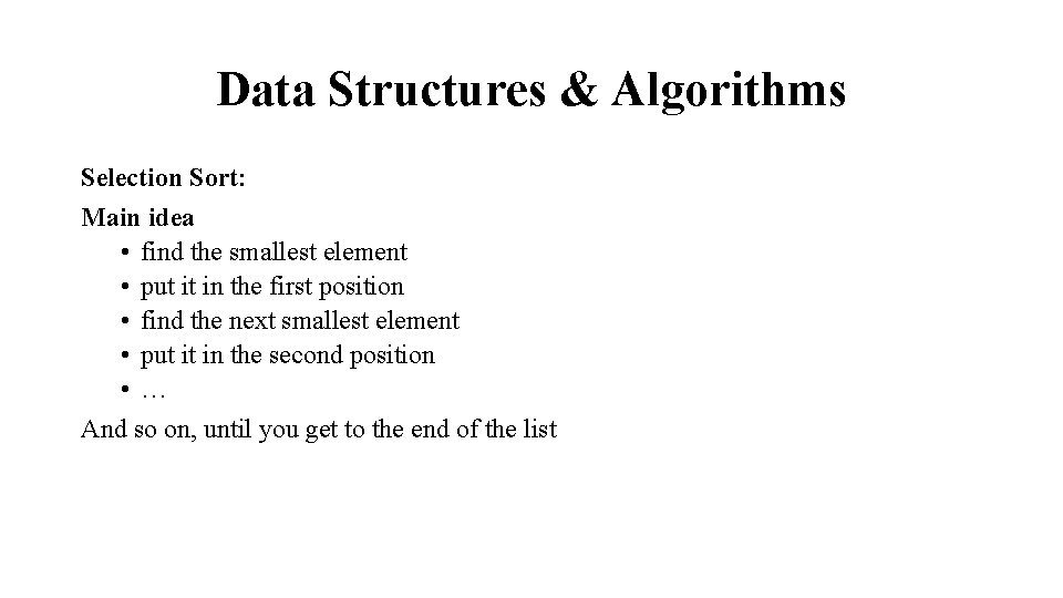
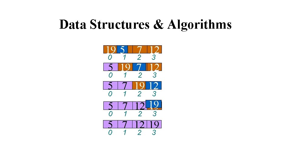
Data Structures & Algorithms Selection Sort: Main idea • find the smallest element • put it in the first position • find the next smallest element • put it in the second position • … And so on, until you get to the end of the list

Data Structures & Algorithms 55 7 12 a 19 0 1 2 3 : 5 19 7 12 0 1 2 3 5 7 19 12 0 1 2 3 5 7 12 19 0 1 2 3

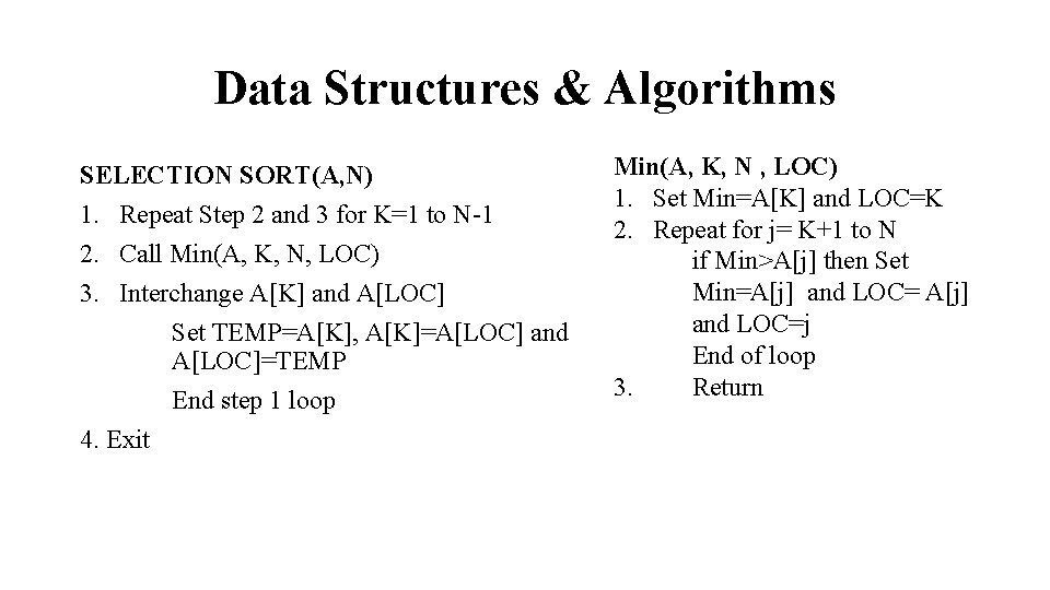
Data Structures & Algorithms SELECTION SORT(A, N) 1. Repeat Step 2 and 3 for K=1 to N-1 2. Call Min(A, K, N, LOC) 3. Interchange A[K] and A[LOC] Set TEMP=A[K], A[K]=A[LOC] and A[LOC]=TEMP End step 1 loop 4. Exit Min(A, K, N , LOC) 1. Set Min=A[K] and LOC=K 2. Repeat for j= K+1 to N if Min>A[j] then Set Min=A[j] and LOC=j End of loop 3. Return

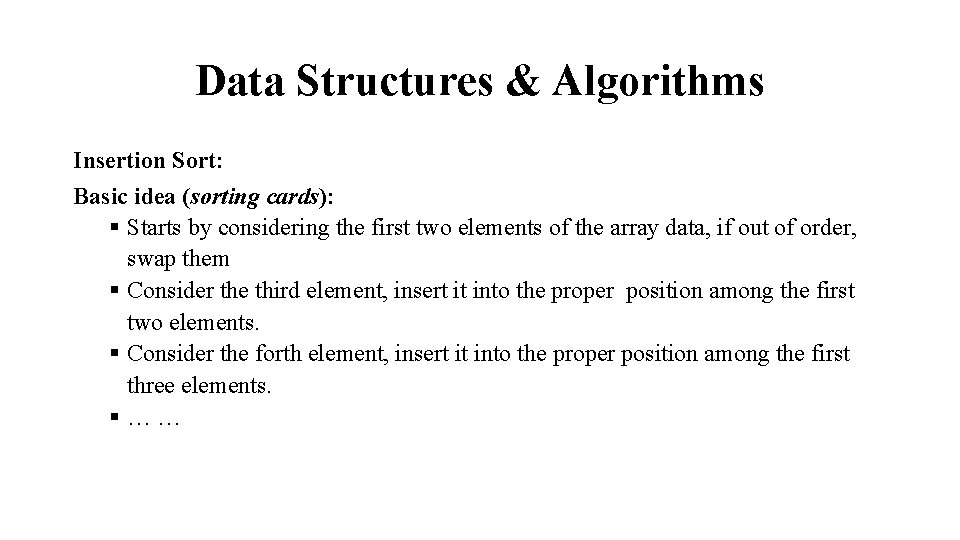
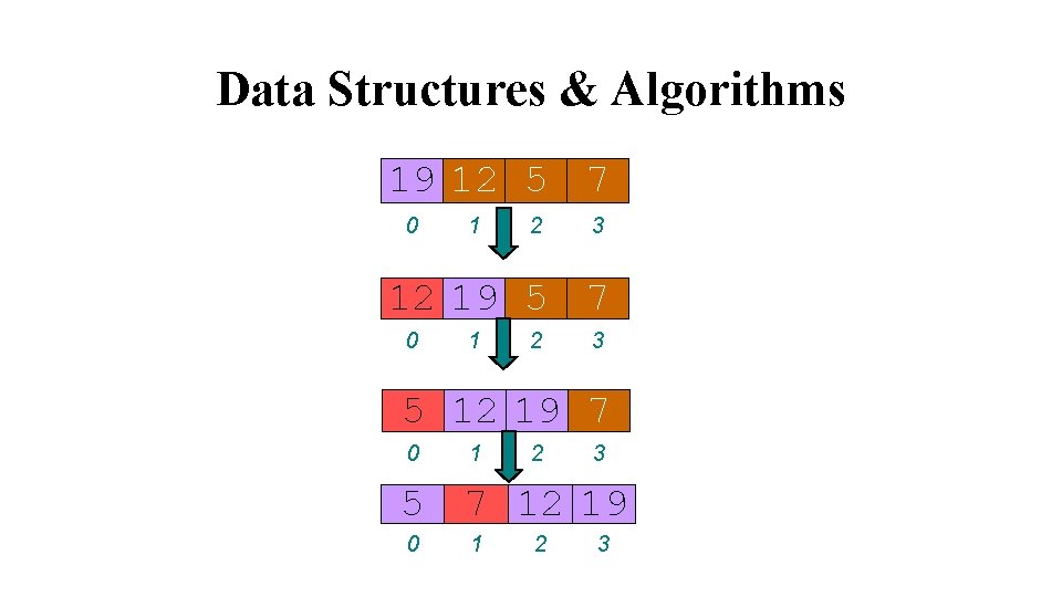
Data Structures & Algorithms Insertion Sort: Basic idea (sorting cards): § Starts by considering the first two elements of the array data, if out of order, swap them § Consider the third element, insert it into the proper position among the first two elements. § Consider the forth element, insert it into the proper position among the first three elements. §……

Data Structures & Algorithms 19 12 5 7 0 1 2 3 12 19 5 7 0 1 2 3 5 12 19 7 0 1 2 3 5 7 12 19 0 1 2 3

Data Structures & Algorithms INSERTION(A, N) 1. Set A[0]= -∞ 2. Repeat 3 to 5 for K=2…. N 3. Set TEMP=A[K] and PTR=K-1 4. Repeat while TEMP<A[PTR] a) Set A[PTR+1]=A[PTR] b) Set PTR=PTR-1 End of Loop 5. Set A[PTR+1]=TEMP End of Loop 6. Return

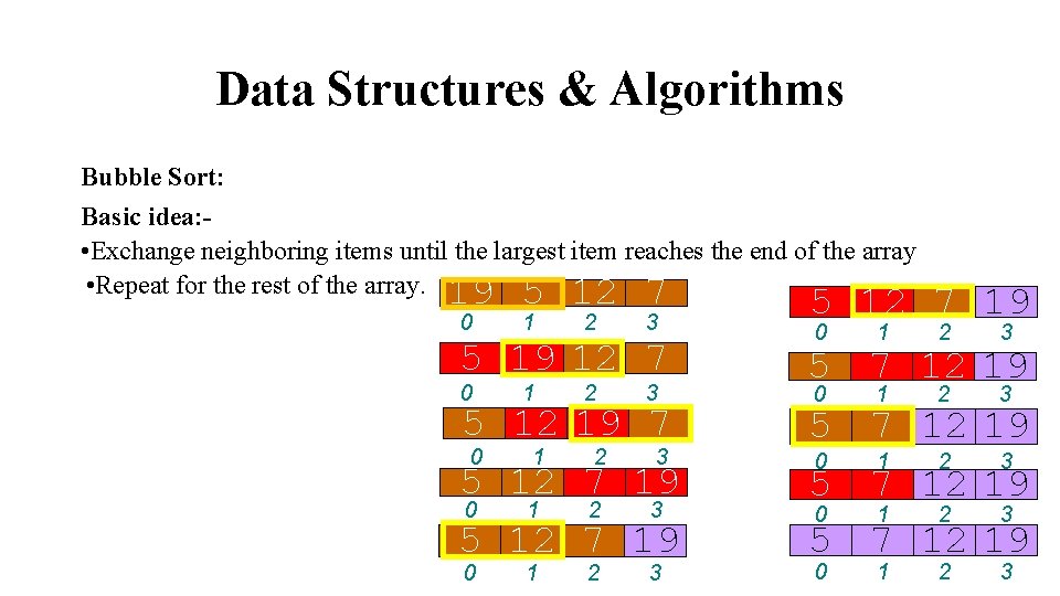
Data Structures & Algorithms Bubble Sort: Basic idea: • Exchange neighboring items until the largest item reaches the end of the array • Repeat for the rest of the array. 19 5 12 7 0 1 2 3 5 19 12 7 0 1 2 3 5 12 19 7 0 1 2 3 5 12 7 19 0 1 2 3 5 0 5 0 5 7 1 7 12 2 12 19 3 19 0 1 2 58 3

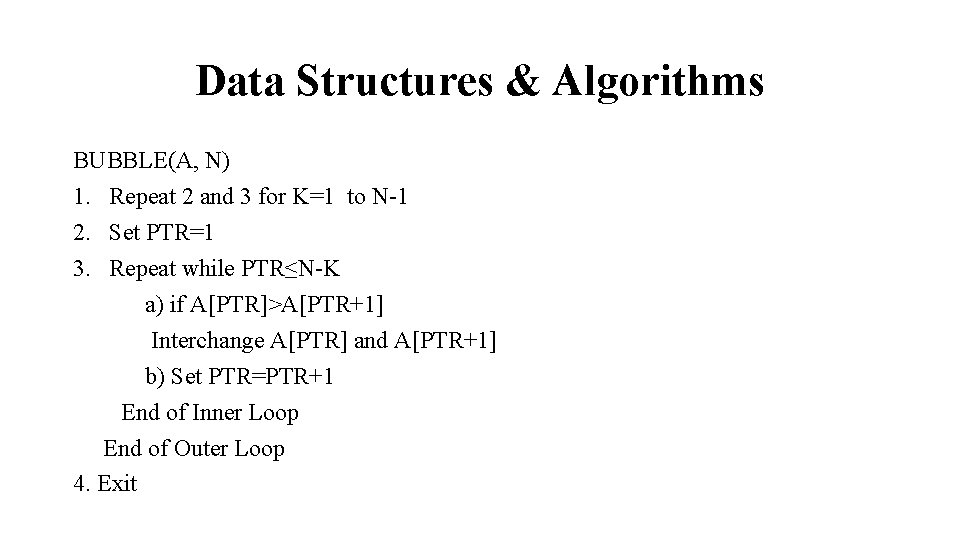
Data Structures & Algorithms BUBBLE(A, N) 1. Repeat 2 and 3 for K=1 to N-1 2. Set PTR=1 3. Repeat while PTR≤N-K a) if A[PTR]>A[PTR+1] Interchange A[PTR] and A[PTR+1] b) Set PTR=PTR+1 End of Inner Loop End of Outer Loop 4. Exit

Data Structures & Algorithms Advance Sorting Algorithms: § Merge Sort § Quick Sort § Heap Sort

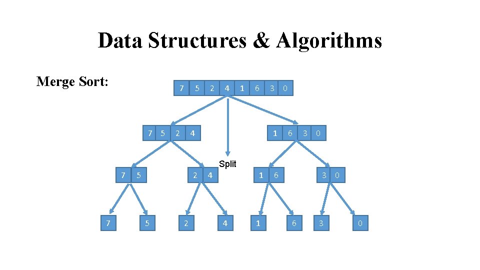
Data Structures & Algorithms Merge Sort: 7 7 5 5 2 2 4 1 6 4 3 0 1 6 3 0 Split 7 7 5 2 4 1 6 3 0

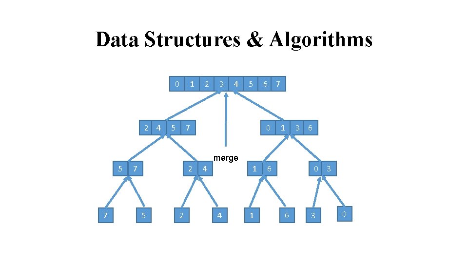
Data Structures & Algorithms 0 2 4 1 5 2 3 4 5 7 6 7 0 1 3 6 merge 5 7 7 2 5 2 4 1 6 0 3 6 3 0

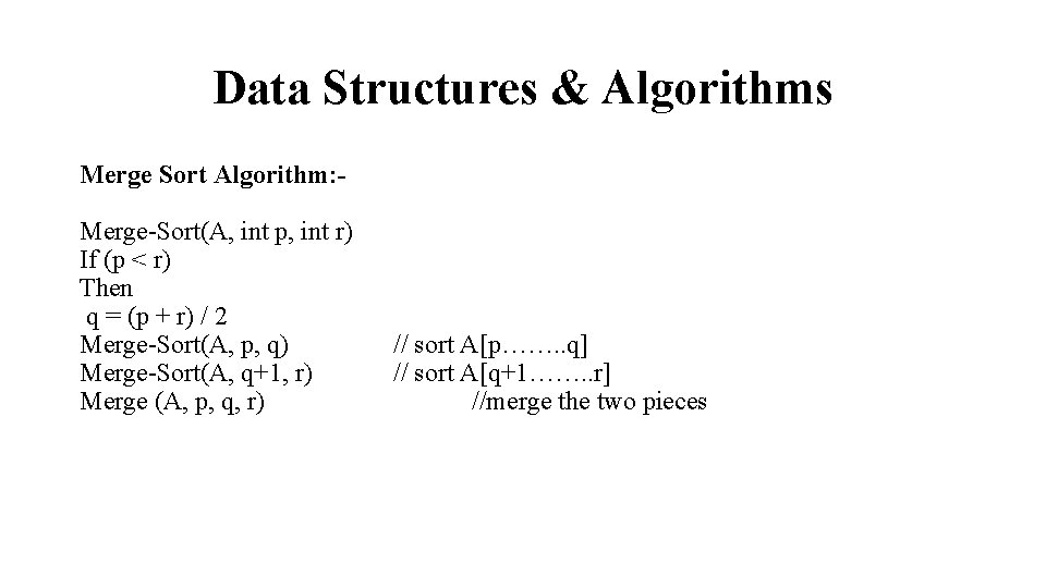
Data Structures & Algorithms Merge Sort Algorithm: Merge-Sort(A, int p, int r) If (p < r) Then q = (p + r) / 2 Merge-Sort(A, p, q) Merge-Sort(A, q+1, r) Merge (A, p, q, r) // sort A[p……. . q] // sort A[q+1……. . r] //merge the two pieces

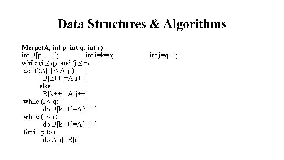
Data Structures & Algorithms Merge(A, int p, int q, int r) int B[p…. . r]; int i=k=p; while (i ≤ q) and (j ≤ r) do if (A[i] ≤ A[j]) B[k++]=A[i++] else B[k++]=A[j++] while (i ≤ q) do B[k++]=A[i++] while (j ≤ r) do B[k++]=A[j++] for i= p to r do A[i]=B[i] int j=q+1;

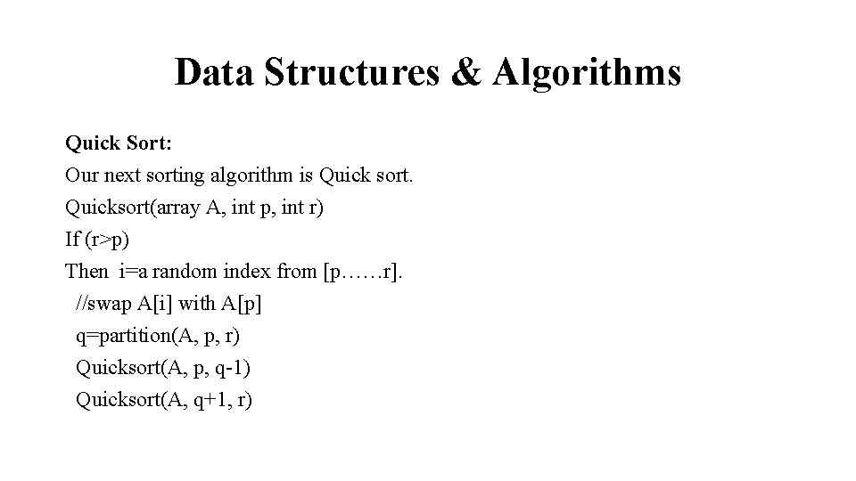
Data Structures & Algorithms Quick Sort: Our next sorting algorithm is Quick sort. Quicksort(array A, int p, int r) If (r>p) Then i=a random index from [p……r]. //swap A[i] with A[p] q=partition(A, p, r) Quicksort(A, p, q-1) Quicksort(A, q+1, r)

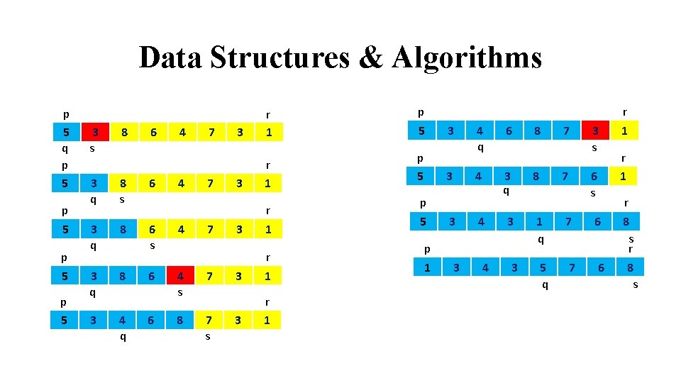
Data Structures & Algorithms We know that partition algorithm partitions the array A[p……r] into three subarrays about a pivot element x. Ø A[p……q-1] whose elements are less than or equal to x. ØA[x] ØA[q+1……r] whose elements are greater than x. We will choose the first element of the array as pivot i. e. x=A[p] We can also choose the pivot element randomly.

Data Structures & Algorithms The algorithm works by maintaining the following invariant conditions. ØA[p]=x is the pivot value. ØA[p……q-1] contain elements that are less than x. ØA[q+1……. s-1] contain elements that are greater than or equal to x. ØA[s……r] contain elements whose values are currently unknown.

Data Structures & Algorithms Partition(array A, int p, int r) x=A[p] q=p for s=p+1 to r { if (A[s]<x) { q=q+1 swap A[q] with A[s] } } swap A[p] with A[q] return q

Data Structures & Algorithms p 5 q p 5 p 5 3 s 8 6 4 3 q 8 s 6 3 q 8 6 s 4 3 q 8 6 4 s 7 3 4 q 8 7 s 6 4 7 7 7 3 r 1 3 r 1 p 5 3 3 p 5 p 1 3 3 4 q 6 4 3 q 4 4 8 8 3 3 7 7 1 q 5 q 3 s 6 s 7 7 6 6 r 1 r 8 s

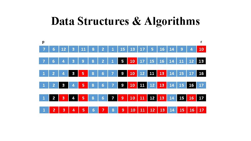
Data Structures & Algorithms p r 7 6 12 3 11 8 2 1 15 13 17 5 16 14 9 4 10 7 6 4 3 9 8 2 1 5 10 17 15 16 14 11 12 13 1 2 4 3 5 8 6 7 9 10 12 11 13 14 15 17 16 1 2 3 4 5 8 6 7 9 10 11 12 13 14 15 16 17 1 2 3 4 5 6 7 8 9 10 11 12 13 14 15 16 17

Data Structures & Algorithms The LIST Data Structure: § The List is among the most generic of data structures. § Real life: a. shopping list, b. groceries list, c. list of people to invite to dinner d. Contact list

Data Structures & Algorithms § § § A list is collection of items that are all of the same type (grocery items, integers, names) The items, or elements of the list, are stored in some particular order It is possible to insert new elements into various positions in the list and remove any element of the list. List is a set of elements in a linear order. For example, data values a 1, a 2, a 3, a 4 can be arranged in a list: (a 3, a 1, a 2, a 4) In this list, a 3, is the first element, a 1 is the second element, and so on The order is important here; this is not just a random collection of elements, it is an ordered collection.

Data Structures & Algorithms Useful operations § create. List(): create a new list (presumably empty) § copy(): set one list to be a copy of another § clear(); clear a list (remove all elements) § insert(X, ? ): Insert element X at a particular position in the list § remove(? ): Remove element at some position in the list § get(? ): Get element at a given position § update(X, ? ): replace the element at a given position with X § find(X): determine if the element X is in the list § length(): return the length of the list.

Data Structures & Algorithms § We need to decide what is meant by “particular position”; we have used “? ” for this. § There are two possibilities: § Use the actual index of element: insert after element 3, get element number 6. This approach is taken by arrays § Use a “current” marker or pointer to refer to a particular position in the list.

Data Structures & Algorithms If we use the “current” marker, the following four methods would be useful: § start(): moves to “current” pointer to the very first element. § tail(): moves to “current” pointer to the very last element. § next(): move the current position forward one element § back(): move the current position backward one element

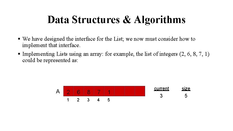
Data Structures & Algorithms § We have designed the interface for the List; we now must consider how to implement that interface. § Implementing Lists using an array: for example, the list of integers (2, 6, 8, 7, 1) could be represented as: A 2 6 8 7 1 1 2 3 4 5 current size 3 5

Data Structures & Algorithms § add(9); current position is 3. The new list would thus be: (2, 6, 8, 9, 7, 1) § We will need to shift everything to the right of 8 one place to the right to make place for the new element ‘ 9’. step 1: step 2: A A 2 6 8 7 1 1 2 3 4 5 6 2 6 8 9 7 1 1 2 3 4 5 6 current size 3 5 current size 4 6 notice: current points to new element

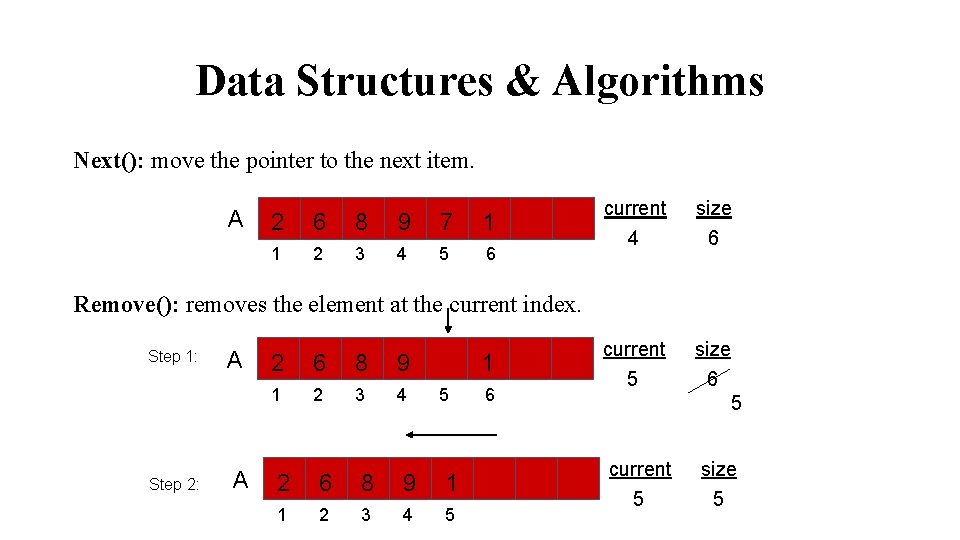
Data Structures & Algorithms Next(): move the pointer to the next item. A 2 6 8 9 7 1 1 2 3 4 5 6 current 4 size current 5 size 6 Remove(): removes the element at the current index. Step 1: Step 2: A A 2 6 8 9 1 2 3 4 1 5 2 6 8 9 1 1 2 3 4 5 6 6 5 current 5 size 5

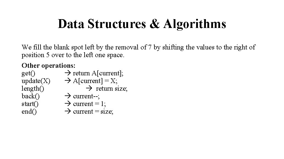
Data Structures & Algorithms We fill the blank spot left by the removal of 7 by shifting the values to the right of position 5 over to the left one space. Other operations: get() return A[current]; update(X) A[current] = X; length() return size; back() current--; start() current = 1; end() current = size;

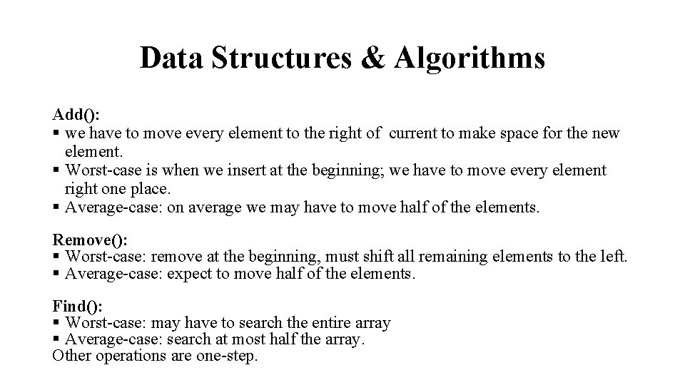
Data Structures & Algorithms Add(): § we have to move every element to the right of current to make space for the new element. § Worst-case is when we insert at the beginning; we have to move every element right one place. § Average-case: on average we may have to move half of the elements. Remove(): § Worst-case: remove at the beginning, must shift all remaining elements to the left. § Average-case: expect to move half of the elements. Find(): § Worst-case: may have to search the entire array § Average-case: search at most half the array. Other operations are one-step.

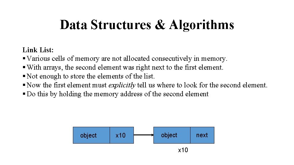
Data Structures & Algorithms Link List: § Various cells of memory are not allocated consecutively in memory. § With arrays, the second element was right next to the first element. § Not enough to store the elements of the list. § Now the first element must explicitly tell us where to look for the second element. § Do this by holding the memory address of the second element object x 10 object next x 10

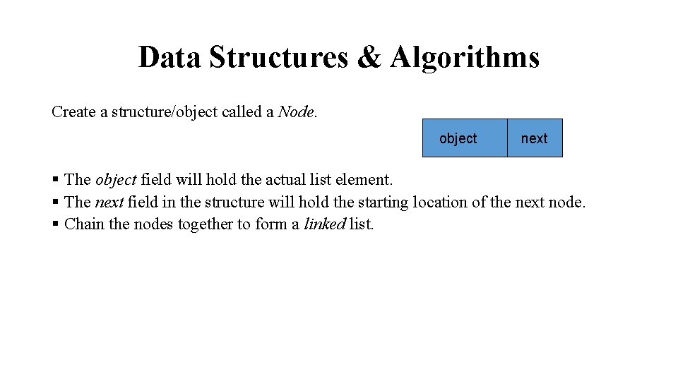
Data Structures & Algorithms Create a structure/object called a Node. object next § The object field will hold the actual list element. § The next field in the structure will hold the starting location of the next node. § Chain the nodes together to form a linked list.

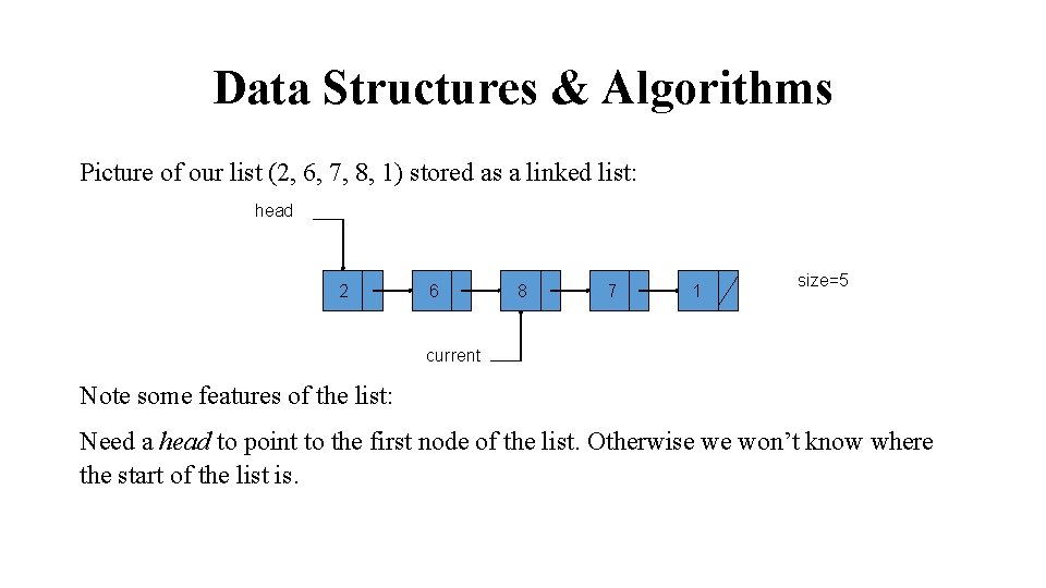
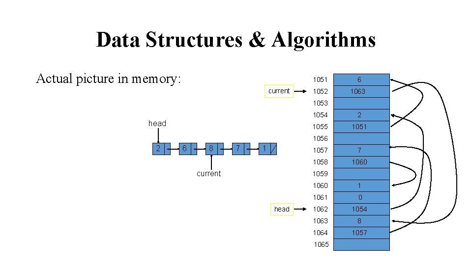
Data Structures & Algorithms Picture of our list (2, 6, 7, 8, 1) stored as a linked list: head 2 6 8 7 1 size=5 current Note some features of the list: Need a head to point to the first node of the list. Otherwise we won’t know where the start of the list is.

Data Structures & Algorithms The current here is a pointer, not an index. The next field in the last node points to nothing. We will place the memory address NULL which is guaranteed to be inaccessible.

Data Structures & Algorithms Actual picture in memory: current 1051 6 1052 1063 1053 head 1054 2 1055 1051 1056 2 6 8 7 1 current 1057 7 1058 1060 1059 head 1060 1 1061 0 1062 1054 1063 8 1064 1057 1065

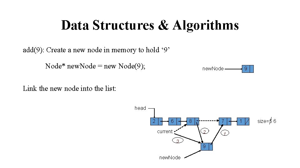
Data Structures & Algorithms add(9): Create a new node in memory to hold ‘ 9’ Node* new. Node = new Node(9); new. Node 9 Link the new node into the list: head 2 6 8 current 7 2 3 9 new. Node 1 1 size=5 6

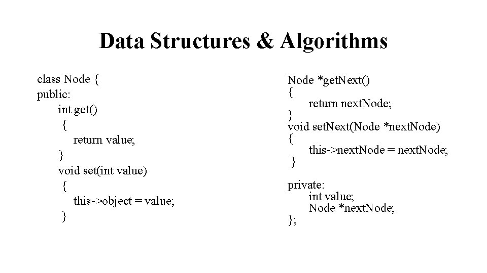
Data Structures & Algorithms class Node { public: int get() { return value; } void set(int value) { this->object = value; } Node *get. Next() { return next. Node; } void set. Next(Node *next. Node) { this->next. Node = next. Node; } private: int value; Node *next. Node; };

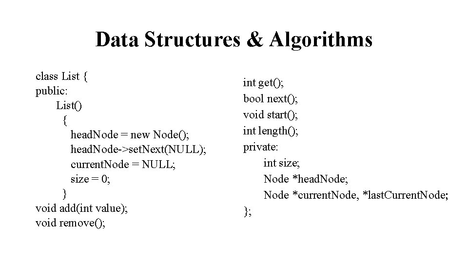
Data Structures & Algorithms class List { public: List() { head. Node = new Node(); head. Node->set. Next(NULL); current. Node = NULL; size = 0; } void add(int value); void remove(); int get(); bool next(); void start(); int length(); private: int size; Node *head. Node; Node *current. Node, *last. Current. Node; };

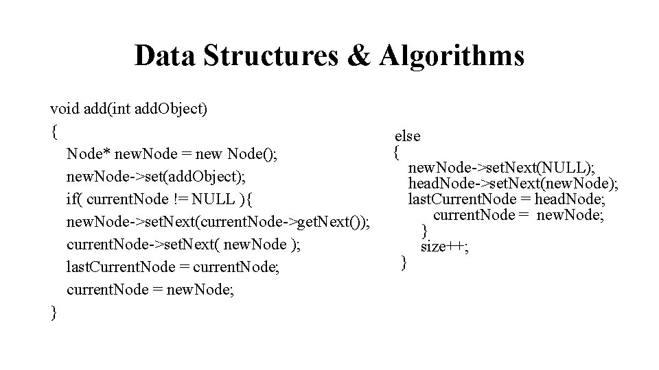
Data Structures & Algorithms void add(int add. Object) { Node* new. Node = new Node(); new. Node->set(add. Object); if( current. Node != NULL ){ new. Node->set. Next(current. Node->get. Next()); current. Node->set. Next( new. Node ); last. Current. Node = current. Node; current. Node = new. Node; } else { new. Node->set. Next(NULL); head. Node->set. Next(new. Node); last. Current. Node = head. Node; current. Node = new. Node; } size++; }

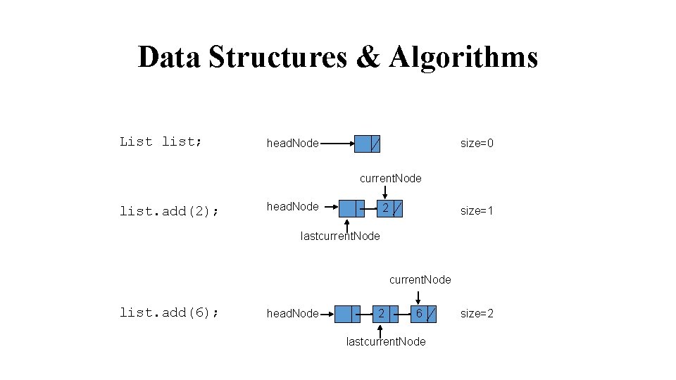
Data Structures & Algorithms List list; head. Node size=0 current. Node list. add(2); head. Node 2 size=1 lastcurrent. Node list. add(6); head. Node 2 6 lastcurrent. Node size=2

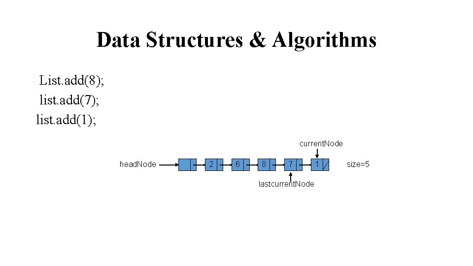
Data Structures & Algorithms List. add(8); list. add(7); list. add(1); current. Node head. Node 2 6 8 7 lastcurrent. Node 1 size=5

Data Structures & Algorithms void remove() { if( current. Node != NULL && current. Node != head. Node) { last. Current. Node->set. Next(current. Node->get. Next()); delete current. Node; current. Node = last. Current. Node->get. Next(); size--; current. Node } head. Node }; 2 6 lastcurrent. Node 8 7 1 size=5

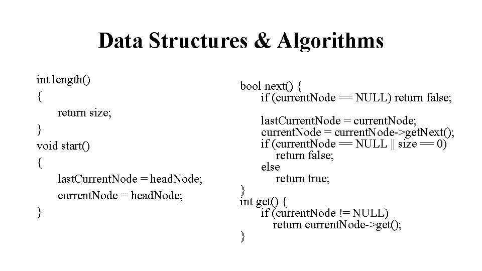
Data Structures & Algorithms int length() { return size; } void start() { last. Current. Node = head. Node; current. Node = head. Node; } bool next() { if (current. Node == NULL) return false; last. Current. Node = current. Node; current. Node = current. Node->get. Next(); if (current. Node == NULL || size == 0) return false; else return true; } int get() { if (current. Node != NULL) return current. Node->get(); }

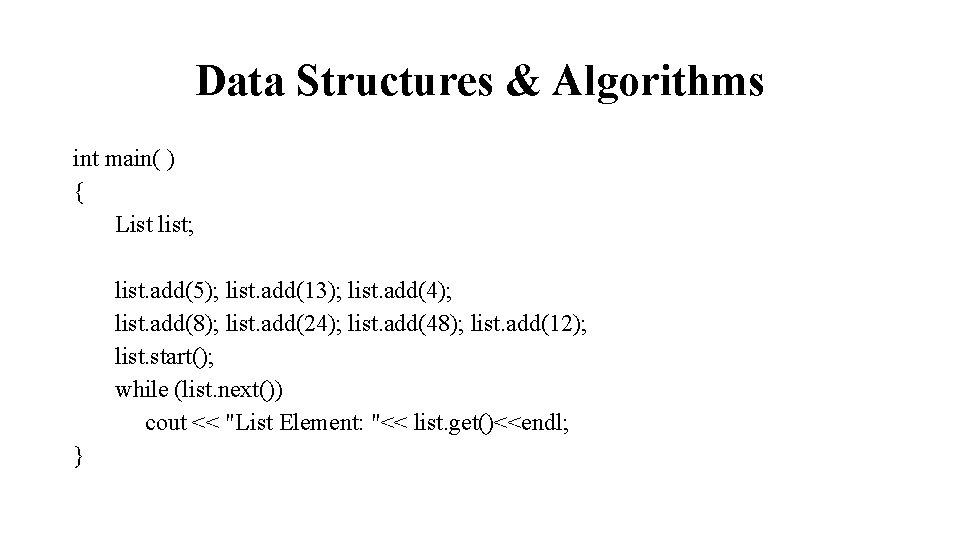
Data Structures & Algorithms int main( ) { List list; list. add(5); list. add(13); list. add(4); list. add(8); list. add(24); list. add(48); list. add(12); list. start(); while (list. next()) cout << "List Element: "<< list. get()<<endl; }

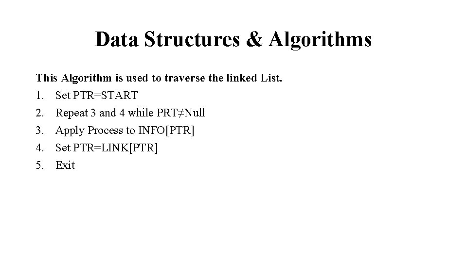
Data Structures & Algorithms This Algorithm is used to traverse the linked List. 1. Set PTR=START 2. Repeat 3 and 4 while PRT≠Null 3. Apply Process to INFO[PTR] 4. Set PTR=LINK[PTR] 5. Exit

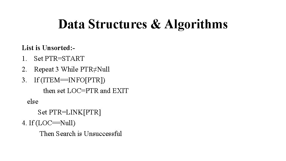
Data Structures & Algorithms List is Unsorted: 1. Set PTR=START 2. Repeat 3 While PTR≠Null 3. If (ITEM==INFO[PTR]) then set LOC=PTR and EXIT else Set PTR=LINK[PTR] 4. If (LOC==Null) Then Search is Unsuccessful

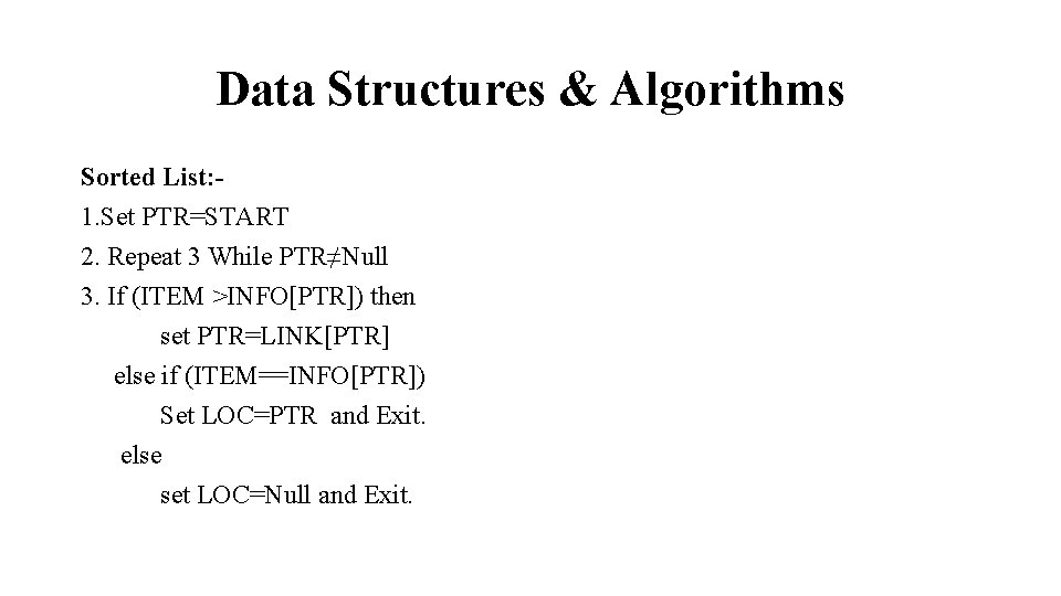
Data Structures & Algorithms Sorted List: 1. Set PTR=START 2. Repeat 3 While PTR≠Null 3. If (ITEM >INFO[PTR]) then set PTR=LINK[PTR] else if (ITEM==INFO[PTR]) Set LOC=PTR and Exit. else set LOC=Null and Exit.

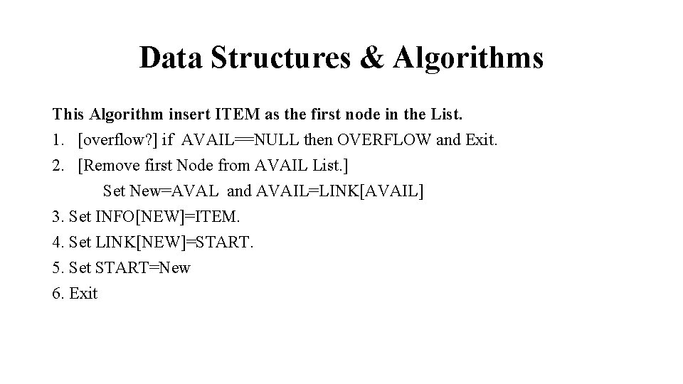
Data Structures & Algorithms This Algorithm insert ITEM as the first node in the List. 1. [overflow? ] if AVAIL==NULL then OVERFLOW and Exit. 2. [Remove first Node from AVAIL List. ] Set New=AVAL and AVAIL=LINK[AVAIL] 3. Set INFO[NEW]=ITEM. 4. Set LINK[NEW]=START. 5. Set START=New 6. Exit

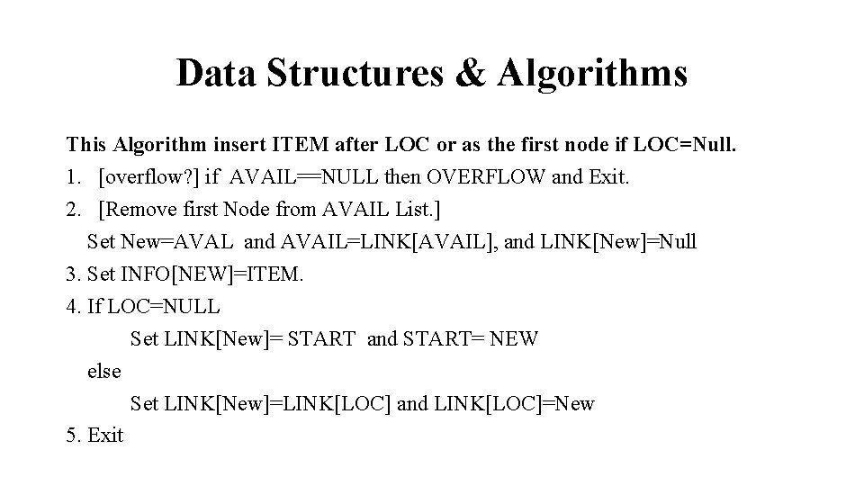
Data Structures & Algorithms This Algorithm insert ITEM after LOC or as the first node if LOC=Null. 1. [overflow? ] if AVAIL==NULL then OVERFLOW and Exit. 2. [Remove first Node from AVAIL List. ] Set New=AVAL and AVAIL=LINK[AVAIL], and LINK[New]=Null 3. Set INFO[NEW]=ITEM. 4. If LOC=NULL Set LINK[New]= START and START= NEW else Set LINK[New]=LINK[LOC] and LINK[LOC]=New 5. Exit

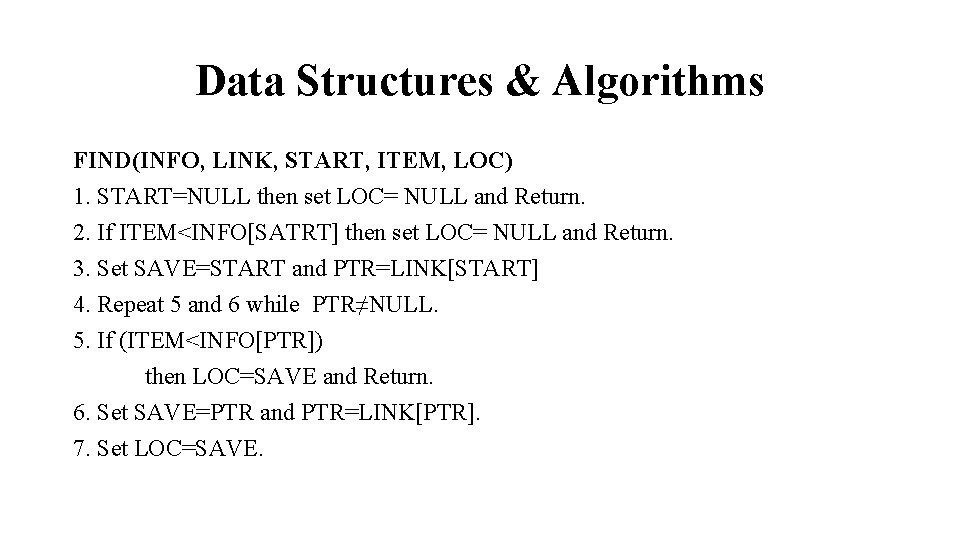
Data Structures & Algorithms FIND(INFO, LINK, START, ITEM, LOC) 1. START=NULL then set LOC= NULL and Return. 2. If ITEM<INFO[SATRT] then set LOC= NULL and Return. 3. Set SAVE=START and PTR=LINK[START] 4. Repeat 5 and 6 while PTR≠NULL. 5. If (ITEM<INFO[PTR]) then LOC=SAVE and Return. 6. Set SAVE=PTR and PTR=LINK[PTR]. 7. Set LOC=SAVE.

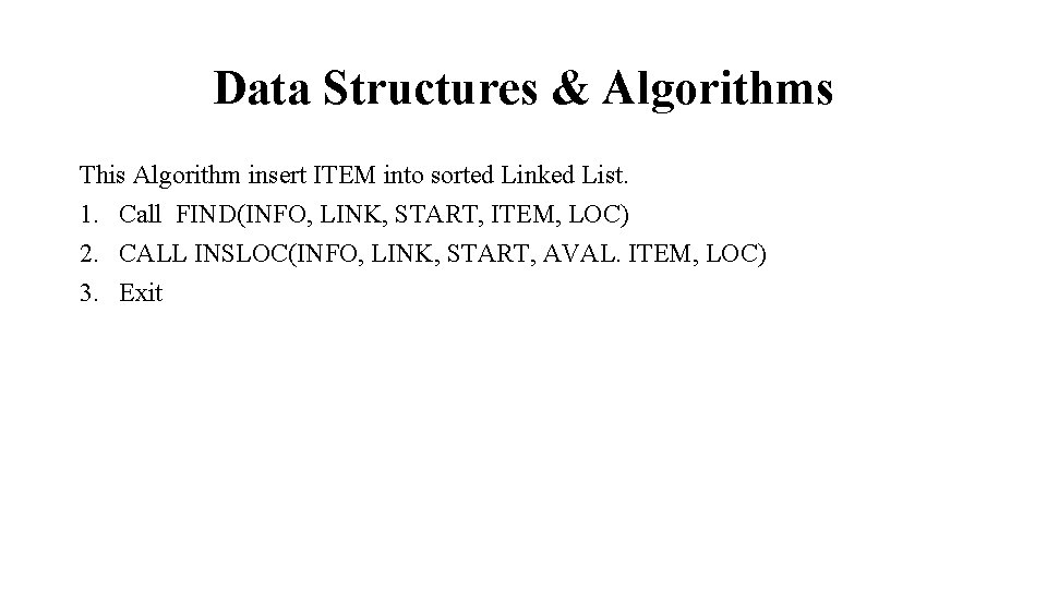
Data Structures & Algorithms This Algorithm insert ITEM into sorted Linked List. 1. Call FIND(INFO, LINK, START, ITEM, LOC) 2. CALL INSLOC(INFO, LINK, START, AVAL. ITEM, LOC) 3. Exit

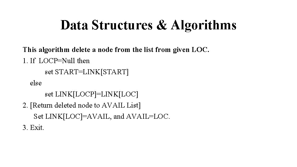
Data Structures & Algorithms This algorithm delete a node from the list from given LOC. 1. If LOCP=Null then set START=LINK[START] else set LINK[LOCP]=LINK[LOC] 2. [Return deleted node to AVAIL List] Set LINK[LOC]=AVAIL, and AVAIL=LOC. 3. Exit.

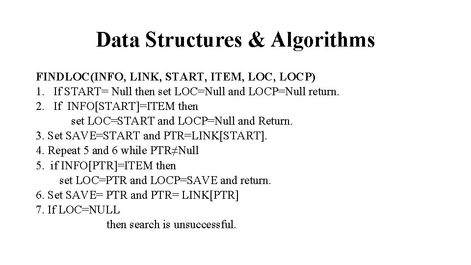
Data Structures & Algorithms FINDLOC(INFO, LINK, START, ITEM, LOCP) 1. If START= Null then set LOC=Null and LOCP=Null return. 2. If INFO[START]=ITEM then set LOC=START and LOCP=Null and Return. 3. Set SAVE=START and PTR=LINK[START]. 4. Repeat 5 and 6 while PTR≠Null 5. if INFO[PTR]=ITEM then set LOC=PTR and LOCP=SAVE and return. 6. Set SAVE= PTR and PTR= LINK[PTR] 7. If LOC=NULL then search is unsuccessful.

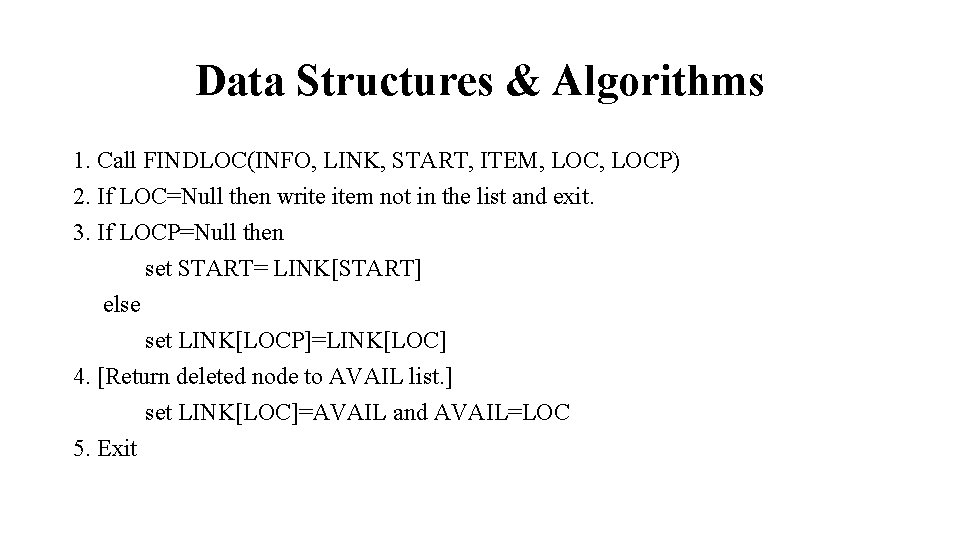
Data Structures & Algorithms 1. Call FINDLOC(INFO, LINK, START, ITEM, LOCP) 2. If LOC=Null then write item not in the list and exit. 3. If LOCP=Null then set START= LINK[START] else set LINK[LOCP]=LINK[LOC] 4. [Return deleted node to AVAIL list. ] set LINK[LOC]=AVAIL and AVAIL=LOC 5. Exit

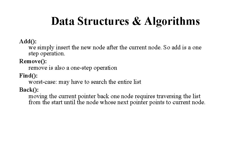
Data Structures & Algorithms Add(): we simply insert the new node after the current node. So add is a one step operation. Remove(): remove is also a one-step operation Find(): worst-case: may have to search the entire list Back(): moving the current pointer back one node requires traversing the list from the start until the node whose next pointer points to current node.

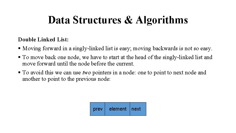
Data Structures & Algorithms Double Linked List: § Moving forward in a singly-linked list is easy; moving backwards is not so easy. § To move back one node, we have to start at the head of the singly-linked list and move forward until the node before the current. § To avoid this we can use two pointers in a node: one to point to next node and another to point to the previous node: prev element next

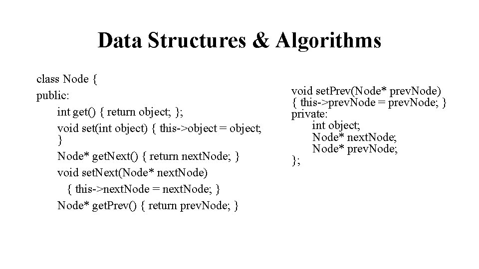
Data Structures & Algorithms class Node { public: int get() { return object; }; void set(int object) { this->object = object; } Node* get. Next() { return next. Node; } void set. Next(Node* next. Node) { this->next. Node = next. Node; } Node* get. Prev() { return prev. Node; } void set. Prev(Node* prev. Node) { this->prev. Node = prev. Node; } private: int object; Node* next. Node; Node* prev. Node; };

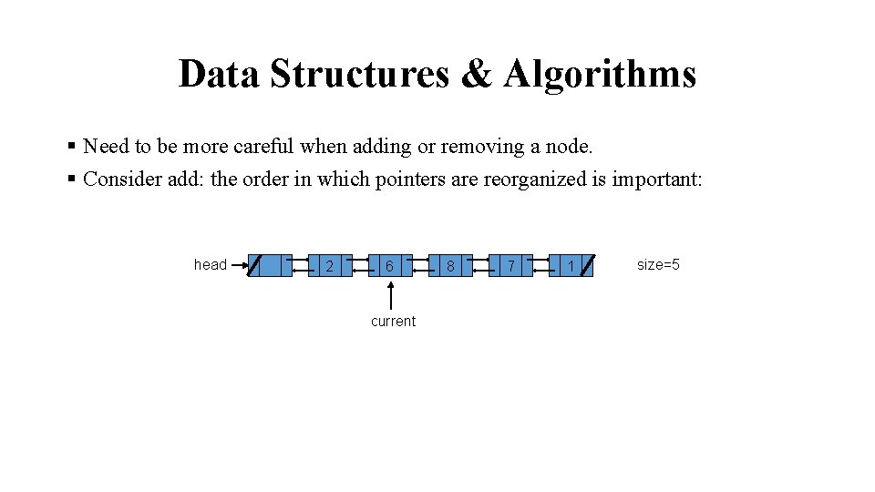
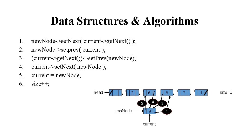
Data Structures & Algorithms § Need to be more careful when adding or removing a node. § Consider add: the order in which pointers are reorganized is important: head 2 6 current 8 7 1 size=5

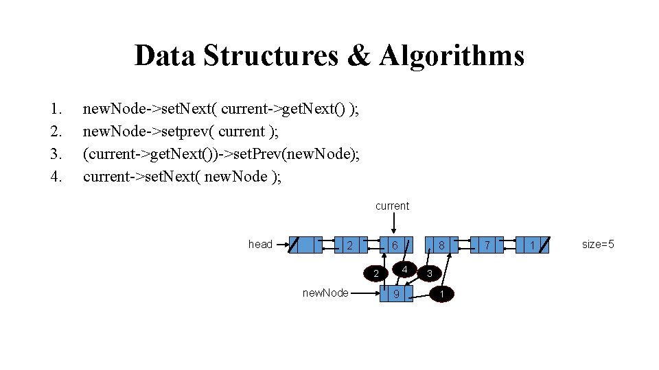
Data Structures & Algorithms 1. 2. 3. 4. new. Node->set. Next( current->get. Next() ); new. Node->setprev( current ); (current->get. Next())->set. Prev(new. Node); current->set. Next( new. Node ); current head 2 6 4 2 new. Node 8 9 3 1 7 1 size=5

Data Structures & Algorithms 1. 2. 3. 4. 5. 6. new. Node->set. Next( current->get. Next() ); new. Node->setprev( current ); (current->get. Next())->set. Prev(new. Node); current->set. Next( new. Node ); current = new. Node; size++; head 2 6 4 2 new. Node 8 9 current 3 1 7 1 size=6

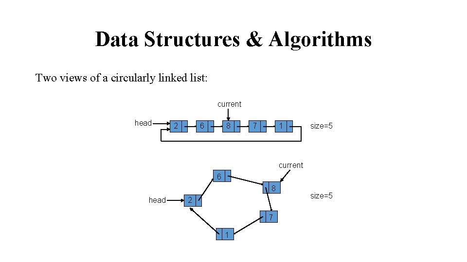
Data Structures & Algorithms § The next field in the last node in a singly-linked list is set to NULL. § Moving along a singly-linked list has to be done in a watchful manner. § Doubly-linked lists have two NULL pointers: prev in the first node and next in the last node. § A way around this potential hazard is to link the last node with the first node in the list to create a circularly-linked list.

Data Structures & Algorithms Two views of a circularly linked list: current head 2 6 8 7 1 size=5 current 6 8 head 2 7 1 size=5