R Data structures Topics covered R data types


![Accessing parts of matrices You may access individual elements by A[x, y], where x Accessing parts of matrices You may access individual elements by A[x, y], where x](https://slidetodoc.com/presentation_image_h2/3ec2949b9bfc987a4c6b38453fab9983/image-32.jpg)


![Subsetting data frames Like matrices, the [i, j]-index notation is valid also for data. Subsetting data frames Like matrices, the [i, j]-index notation is valid also for data.](https://slidetodoc.com/presentation_image_h2/3ec2949b9bfc987a4c6b38453fab9983/image-41.jpg)

![List slicing We retrieve a list slice with the single square bracket "[]" operator. List slicing We retrieve a list slice with the single square bracket "[]" operator.](https://slidetodoc.com/presentation_image_h2/3ec2949b9bfc987a4c6b38453fab9983/image-45.jpg)
![List member reference List entities can be access via double brackets [[]]. This is List member reference List entities can be access via double brackets [[]]. This is](https://slidetodoc.com/presentation_image_h2/3ec2949b9bfc987a4c6b38453fab9983/image-47.jpg)
![List member reference The use of [[]] allows us to change values inside x List member reference The use of [[]] allows us to change values inside x](https://slidetodoc.com/presentation_image_h2/3ec2949b9bfc987a4c6b38453fab9983/image-48.jpg)

- Slides: 76

R Data structures

Topics covered • • • R data types Data structures in R Vectors Matrices Data frames Lists Factors Importing data into R Special programmatic elements

R DATA TYPES revisiting

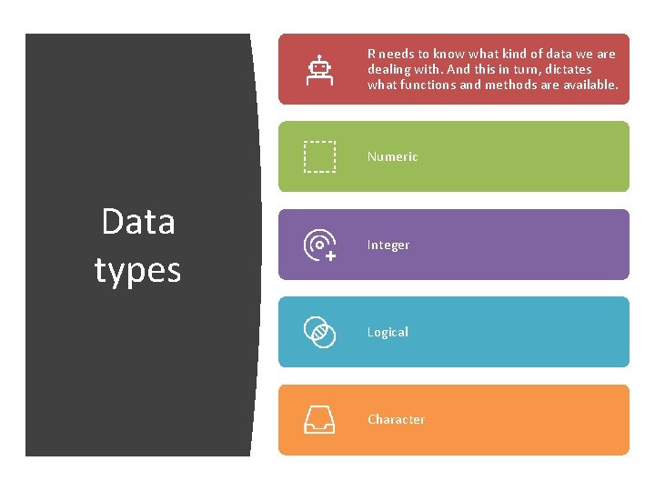
R needs to know what kind of data we are dealing with. And this in turn, dictates what functions and methods are available. Numeric Data types Integer Logical Character

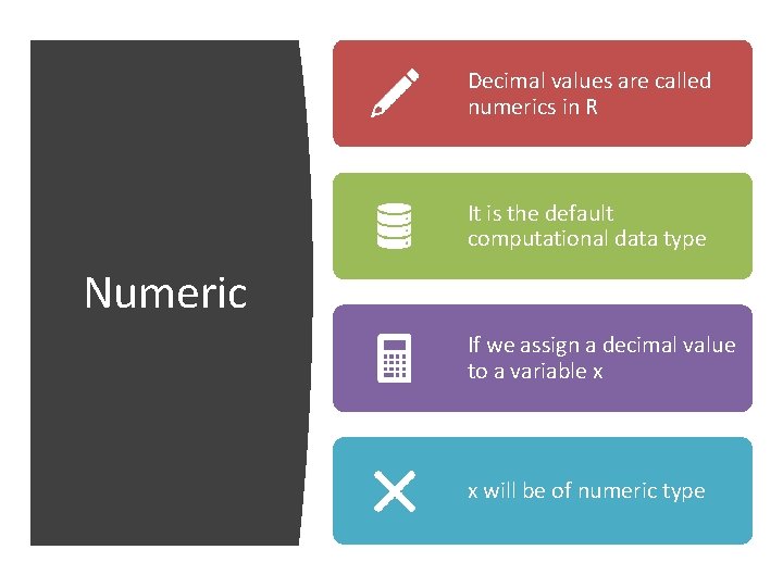
Decimal values are called numerics in R It is the default computational data type Numeric If we assign a decimal value to a variable x x will be of numeric type

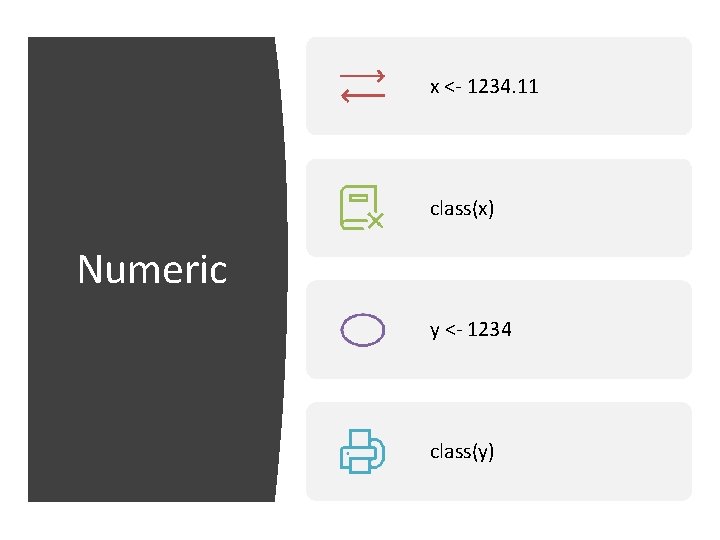
x <- 1234. 11 class(x) Numeric y <- 1234 class(y)

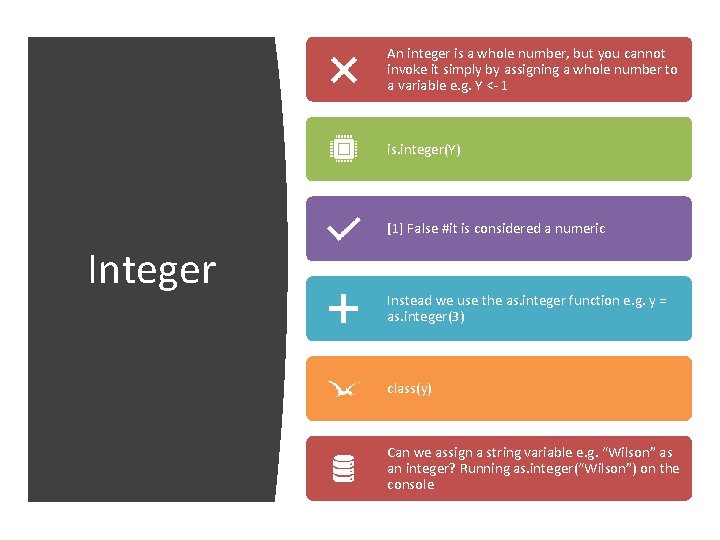
An integer is a whole number, but you cannot invoke it simply by assigning a whole number to a variable e. g. Y <- 1 is. integer(Y) [1] False #it is considered a numeric Integer Instead we use the as. integer function e. g. y = as. integer(3) class(y) Can we assign a string variable e. g. “Wilson” as an integer? Running as. integer(“Wilson”) on the console

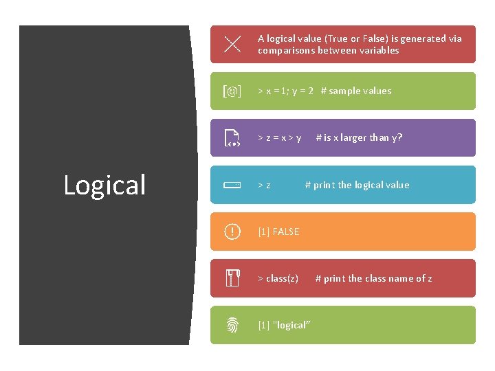
A logical value (True or False) is generated via comparisons between variables > x = 1; y = 2 # sample values >z=x>y Logical >z # is x larger than y? # print the logical value [1] FALSE > class(z) [1] "logical” # print the class name of z

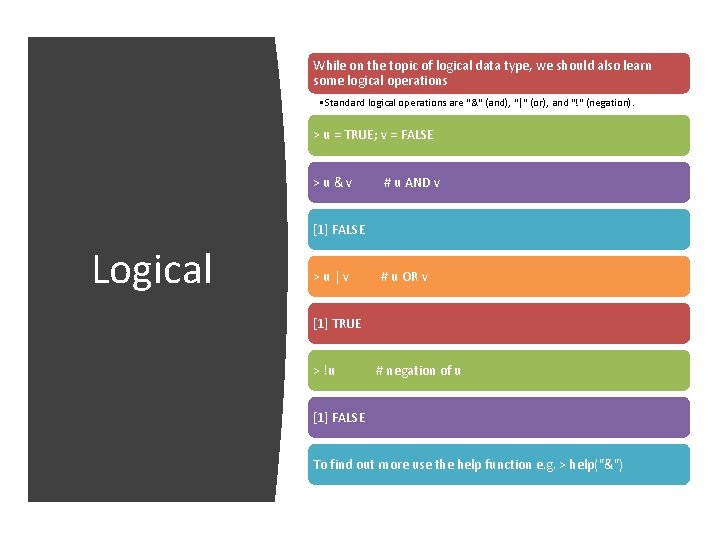
While on the topic of logical data type, we should also learn some logical operations • Standard logical operations are "&" (and), "|" (or), and "!" (negation). > u = TRUE; v = FALSE >u&v # u AND v [1] FALSE Logical >u|v # u OR v [1] TRUE > !u # negation of u [1] FALSE To find out more use the help function e. g. > help("&")

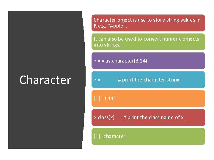
Character object is use to store string values in R e. g. “Apple”. It can also be used to convert numeric objects into strings. > x = as. character(3. 14) Character >x # print the character string [1] "3. 14" > class(x) # print the class name of x [1] "character"

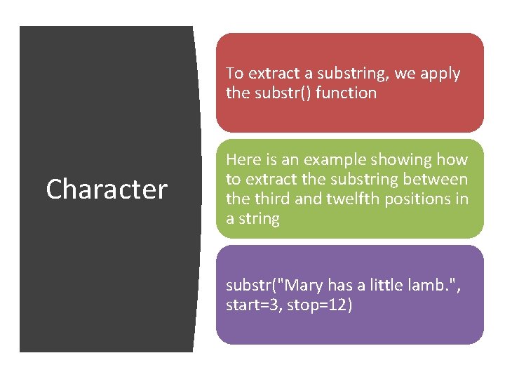
To extract a substring, we apply the substr() function Character Here is an example showing how to extract the substring between the third and twelfth positions in a string substr("Mary has a little lamb. ", start=3, stop=12)

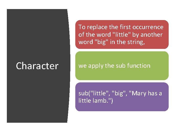
To replace the first occurrence of the word "little" by another word "big" in the string, Character we apply the sub function sub("little", "big", "Mary has a little lamb. ")

DATA STRUCTURES IN R

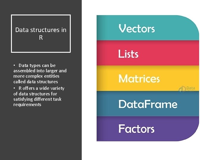
Data structures in R • Data types can be assembled into larger and more complex entities called data structures • R offers a wide variety of data structures for satisfying different task requirements

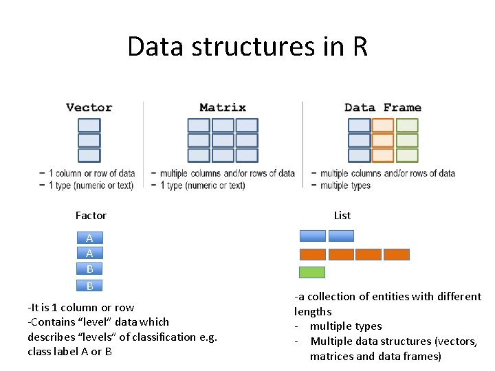
Data structures in R Factor A A B B -It is 1 column or row -Contains “level” data which describes “levels” of classification e. g. class label A or B List -a collection of entities with different lengths - multiple types - Multiple data structures (vectors, matrices and data frames)

VECTORS Vectors

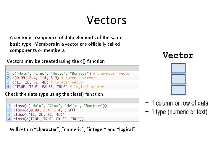
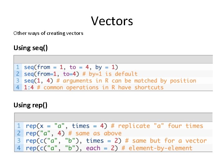
Vectors A vector is a sequence of data elements of the same basic type. Members in a vector are officially called components or members. Vectors may be created using the c() function Check the data type using the class() function Will return “character”, “numeric”, “integer” and “logical”

Vectors Other ways of creating vectors Using seq() Using rep()

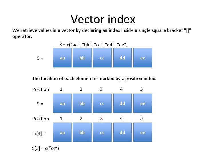
Vector index We retrieve values in a vector by declaring an index inside a single square bracket "[]" operator. S = c("aa", "bb", "cc", "dd", "ee") S= aa bb cc dd ee The location of each element is marked by a position index. Position 1 2 3 4 5 S= aa bb cc dd ee Position 1 2 3 4 5 S[3] = aa bb cc dd ee S[3] = c(“cc”)

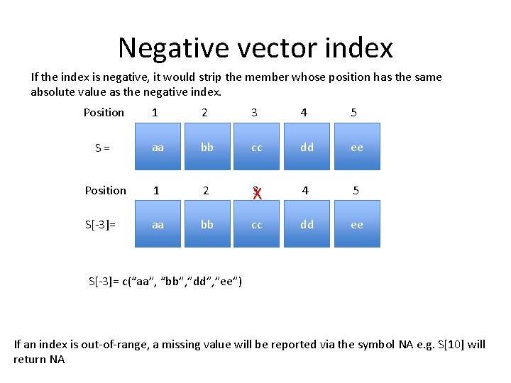
Negative vector index If the index is negative, it would strip the member whose position has the same absolute value as the negative index. Position 1 2 3 4 5 S= aa bb cc dd ee Position 1 2 3 X 4 5 S[-3]= aa bb cc dd ee S[-3]= c(“aa”, “bb”, ”dd”, ”ee”) If an index is out-of-range, a missing value will be reported via the symbol NA e. g. S[10] will return NA

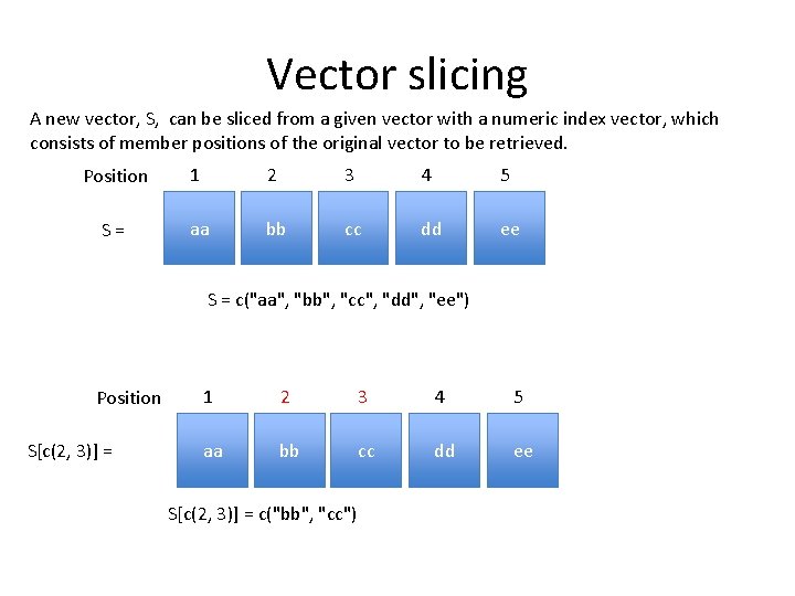
Vector slicing A new vector, S, can be sliced from a given vector with a numeric index vector, which consists of member positions of the original vector to be retrieved. Position 1 2 3 4 5 S= aa bb cc dd ee S = c("aa", "bb", "cc", "dd", "ee") Position S[c(2, 3)] = 1 2 3 4 5 aa bb cc dd ee S[c(2, 3)] = c("bb", "cc")

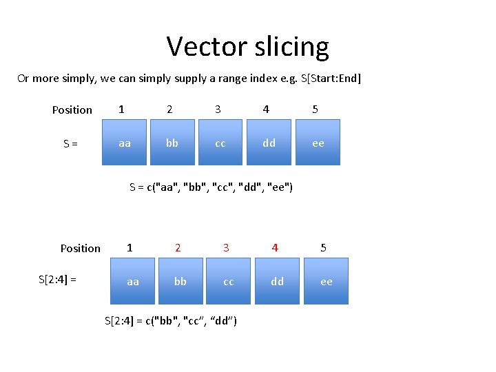
Vector slicing Or more simply, we can simply supply a range index e. g. S[Start: End] Position 1 2 3 4 5 S= aa bb cc dd ee S = c("aa", "bb", "cc", "dd", "ee") Position S[2: 4] = 1 2 3 4 5 aa bb cc dd ee S[2: 4] = c("bb", "cc”, “dd”)

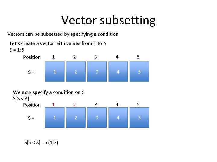
Vector subsetting Vectors can be subsetted by specifying a condition Let’s create a vector with values from 1 to 5 S = 1: 5 1 2 3 Position S= 1 2 We now specify a condition on S S[S < 3] 1 2 Position S= 1 S[S < 3] = c(1, 2) 2 4 5 3 4 5

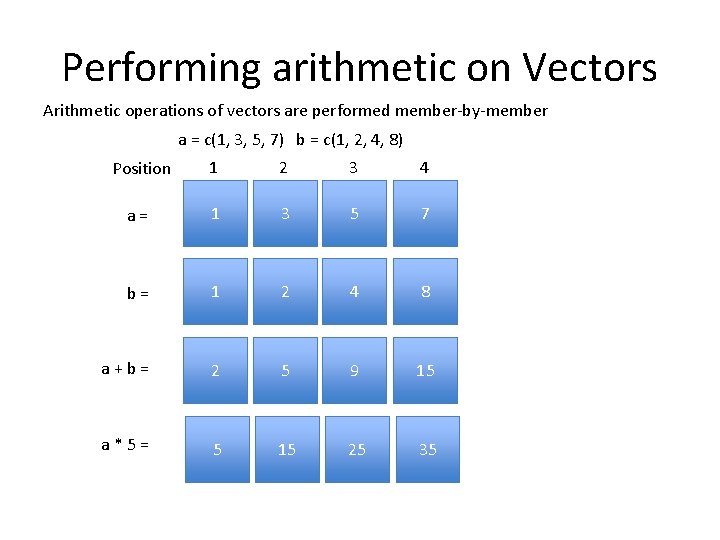
Performing arithmetic on Vectors Arithmetic operations of vectors are performed member-by-member a = c(1, 3, 5, 7) b = c(1, 2, 4, 8) Position 1 2 3 4 a= 1 3 5 7 b= 1 2 4 8 a+b= 2 5 9 15 a*5= 5 15 25 35

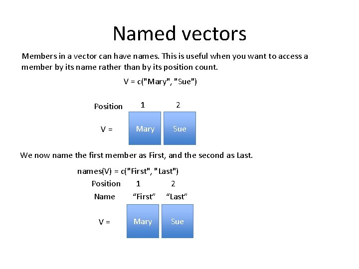
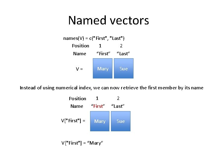
Named vectors Members in a vector can have names. This is useful when you want to access a member by its name rather than by its position count. V = c("Mary", "Sue") Position 1 2 V= Mary Sue We now name the first member as First, and the second as Last. names(V) = c("First", "Last") 1 2 Position Name “First” “Last” V= Mary Sue

Named vectors names(V) = c("First", "Last") 1 2 Position Name “First” “Last” V= Mary Sue Instead of using numerical index, we can now retrieve the first member by its name 1 Position Name “First” V["First"] = Mary V["First"] = “Mary” 2 “Last” Sue

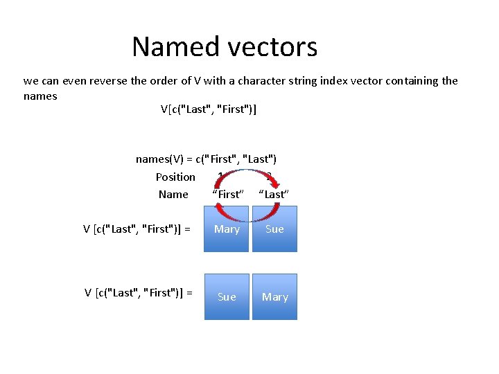
Named vectors we can even reverse the order of V with a character string index vector containing the names V[c("Last", "First")] names(V) = c("First", "Last") 1 2 Position Name “First” “Last” V [c("Last", "First")] = Mary Sue V [c("Last", "First")] = Sue Mary

MATRICES

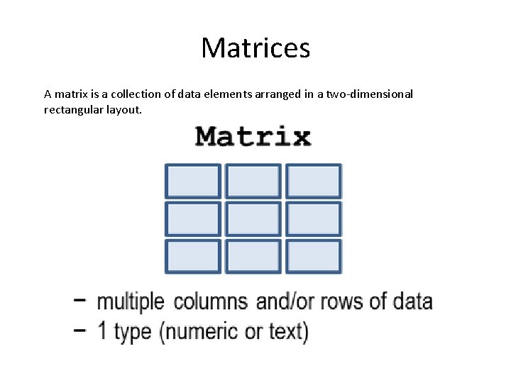
Matrices A matrix is a collection of data elements arranged in a two-dimensional rectangular layout.

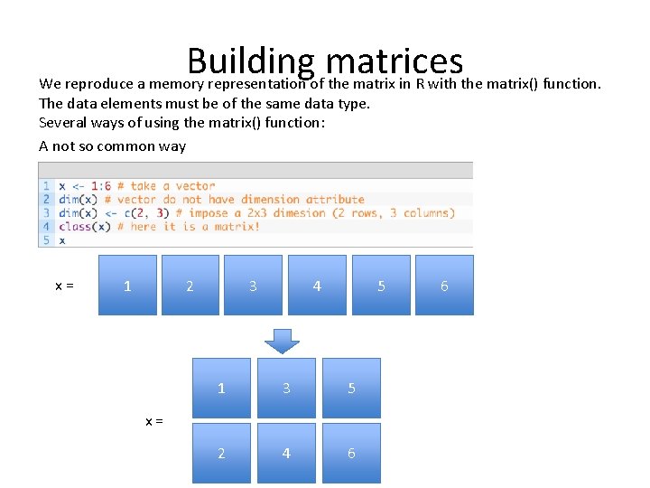
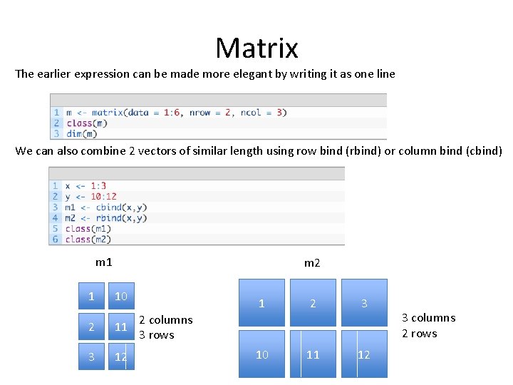
Building matrices We reproduce a memory representation of the matrix in R with the matrix() function. The data elements must be of the same data type. Several ways of using the matrix() function: A not so common way x= 1 2 3 4 5 1 3 5 2 4 6 x= 6

Matrix The earlier expression can be made more elegant by writing it as one line We can also combine 2 vectors of similar length using row bind (rbind) or column bind (cbind) m 1 m 2 1 10 2 11 3 12 1 2 3 10 11 12 2 columns 3 rows 3 columns 2 rows
![Accessing parts of matrices You may access individual elements by Ax y where x Accessing parts of matrices You may access individual elements by A[x, y], where x](https://slidetodoc.com/presentation_image_h2/3ec2949b9bfc987a4c6b38453fab9983/image-32.jpg)
Accessing parts of matrices You may access individual elements by A[x, y], where x is the row number and y is the column number. 1 2 3 A= 1 2 3 10 11 12 A[, 1: 3]= 10 11 12 3 A[2, ] = 10 11 12 A[, 3] = 12

FACTORS

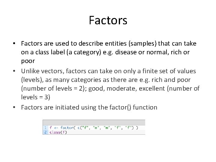
Factors • Factors are used to describe entities (samples) that can take on a class label (a category) e. g. disease or normal, rich or poor • Unlike vectors, factors can take on only a finite set of values (levels), as many categories as there are e. g. rich and poor (number of levels = 2); good, moderate, excellent (number of levels = 3) • Factors are initiated using the factor() function

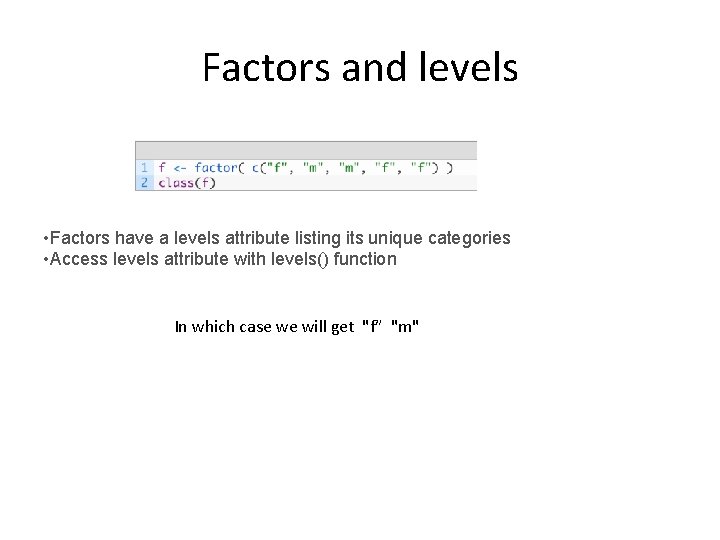
Factors and levels • Factors have a levels attribute listing its unique categories • Access levels attribute with levels() function In which case we will get "f” "m"

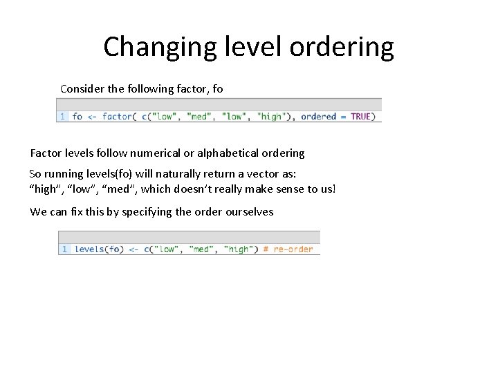
Changing level ordering Consider the following factor, fo Factor levels follow numerical or alphabetical ordering So running levels(fo) will naturally return a vector as: “high”, “low”, “med”, which doesn’t really make sense to us! We can fix this by specifying the order ourselves

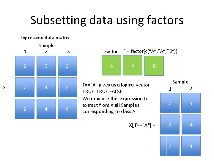
Subsetting data using factors Expression data matrix Sample 2 3 1 2 X= 2 2 3 4 4 5 6 6 Factor F = factor(c(“A”, ”B”)) A A B F=="A” gives us a logical vector TRUE FALSE We may use this expression to extract from X all Samples corresponding to class A X[, F=="A"] = Sample 1 2 2 3 2 4

DATA FRAMES

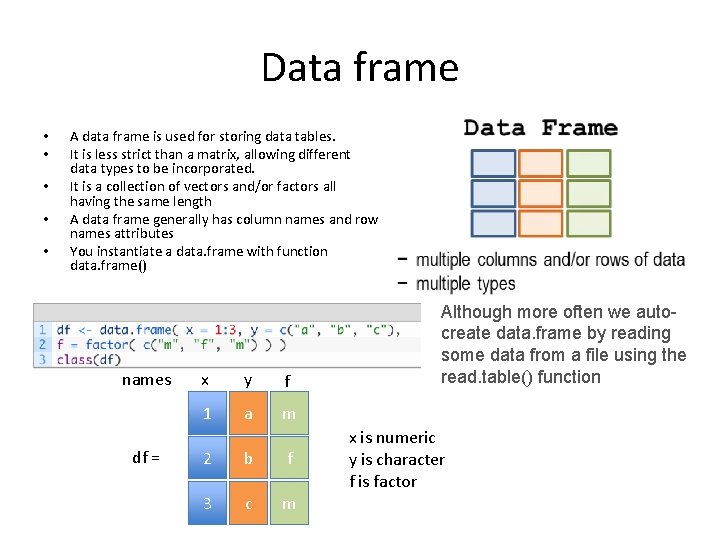
Data frame • • • A data frame is used for storing data tables. It is less strict than a matrix, allowing different data types to be incorporated. It is a collection of vectors and/or factors all having the same length A data frame generally has column names and row names attributes You instantiate a data. frame with function data. frame() names df = x y f 1 a m 2 b f 3 c m Although more often we autocreate data. frame by reading some data from a file using the read. table() function x is numeric y is character f is factor

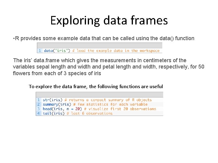
Exploring data frames • R provides some example data that can be called using the data() function The iris’ data. frame which gives the measurements in centimeters of the variables sepal length and width and petal length and width, respectively, for 50 flowers from each of 3 species of iris To explore the data frame, the following functions are useful
![Subsetting data frames Like matrices the i jindex notation is valid also for data Subsetting data frames Like matrices, the [i, j]-index notation is valid also for data.](https://slidetodoc.com/presentation_image_h2/3ec2949b9bfc987a4c6b38453fab9983/image-41.jpg)
Subsetting data frames Like matrices, the [i, j]-index notation is valid also for data. frames names df = x y f 1 a m 2 b f 3 c m 1 df[, 1] = 2 3 df[2, 2] = b

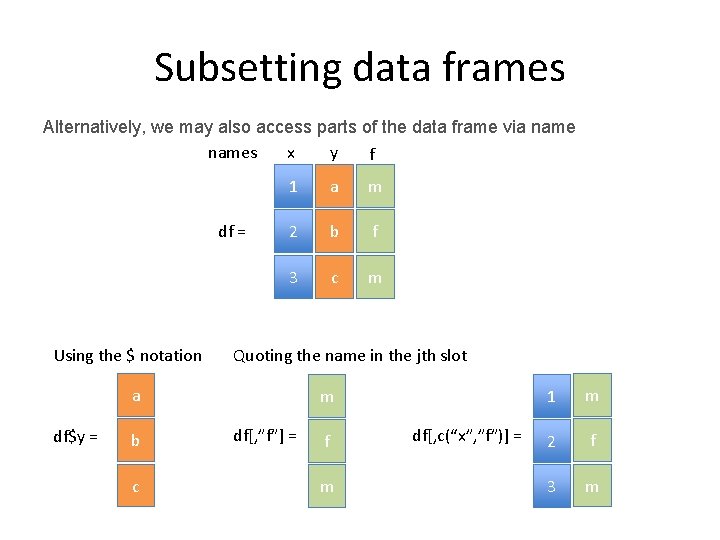
Subsetting data frames Alternatively, we may also access parts of the data frame via names x y f df = Using the $ notation 1 a m 2 b f 3 c m Quoting the name in the jth slot a df$y = b c m df[, ”f”] = f m df[, c(“x”, ”f”)] = 1 m 2 f 3 m

LISTS

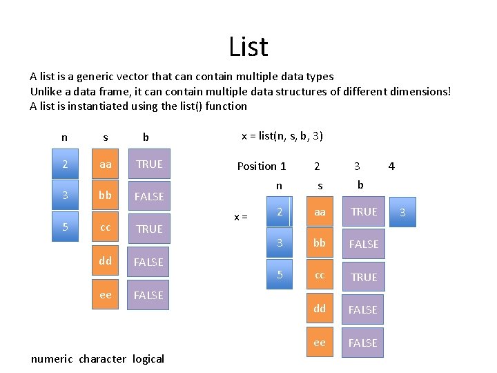
List A list is a generic vector that can contain multiple data types Unlike a data frame, it can contain multiple data structures of different dimensions! A list is instantiated using the list() function n s b 2 aa TRUE 3 5 bb cc dd ee x = list(n, s, b, 3) Position 1 2 3 n s b 2 aa TRUE 3 bb FALSE 5 cc TRUE dd FALSE ee FALSE TRUE FALSE numeric character logical x= 4 3
![List slicing We retrieve a list slice with the single square bracket operator List slicing We retrieve a list slice with the single square bracket "[]" operator.](https://slidetodoc.com/presentation_image_h2/3ec2949b9bfc987a4c6b38453fab9983/image-45.jpg)
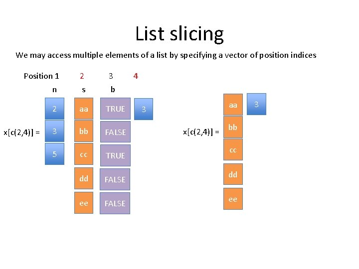
List slicing We retrieve a list slice with the single square bracket "[]" operator. The following is a slice containing the second member of x, which is a copy of s. Position 1 2 3 n s b 2 aa TRUE 3 bb FALSE 5 cc TRUE dd FALSE dd ee FALSE ee x[2] = 4 aa 3 x[2] = bb cc

List slicing We may access multiple elements of a list by specifying a vector of position indices Position 1 2 3 n s b 2 aa TRUE 3 bb FALSE 5 cc TRUE dd FALSE ee FALSE x[c(2, 4)] = 4 aa 3 x[c(2, 4)] = bb cc dd ee 3
![List member reference List entities can be access via double brackets This is List member reference List entities can be access via double brackets [[]]. This is](https://slidetodoc.com/presentation_image_h2/3ec2949b9bfc987a4c6b38453fab9983/image-47.jpg)
List member reference List entities can be access via double brackets [[]]. This is a member reference, and allows us to access a part of the list instead of subsetting it as a separate entity Position 1 x[[2]] = 2 3 4 n s b 2 aa TRUE 3 bb FALSE 5 cc TRUE dd FALSE ee FALSE 3
![List member reference The use of allows us to change values inside x List member reference The use of [[]] allows us to change values inside x](https://slidetodoc.com/presentation_image_h2/3ec2949b9bfc987a4c6b38453fab9983/image-48.jpg)
List member reference The use of [[]] allows us to change values inside x Position 1 x[[2]] = 2 3 4 n s b 2 aa TRUE 3 bb FALSE 5 cc TRUE dd ee Position 1 2 3 4 n s b 2 ta TRUE 3 bb FALSE 5 cc TRUE FALSE dd FALSE ee FALSE 3 x[[2]][1] = "ta” = We access list element 2, at its first position. And changed its value 3

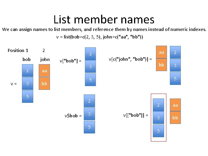
List member names We can assign names to list members, and reference them by names instead of numeric indexes. v = list(bob=c(2, 3, 5), john=c("aa", "bb")) Position 1 bob 2 v= 3 2 john 2 v["bob"] = aa v[c("john", "bob")] = 3 aa 2 bb 3 5 5 bb 5 2 v$bob = 3 5 v[["bob"]] = 2 aa 3 bb 5

IMPORTING DATA INTO R

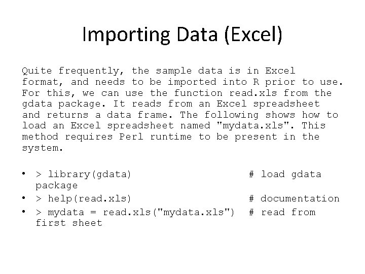
Importing Data (Excel) Quite frequently, the sample data is in Excel format, and needs to be imported into R prior to use. For this, we can use the function read. xls from the gdata package. It reads from an Excel spreadsheet and returns a data frame. The following shows how to load an Excel spreadsheet named "mydata. xls". This method requires Perl runtime to be present in the system. • > library(gdata) package • > help(read. xls) • > mydata = read. xls("mydata. xls") first sheet # load gdata # documentation # read from

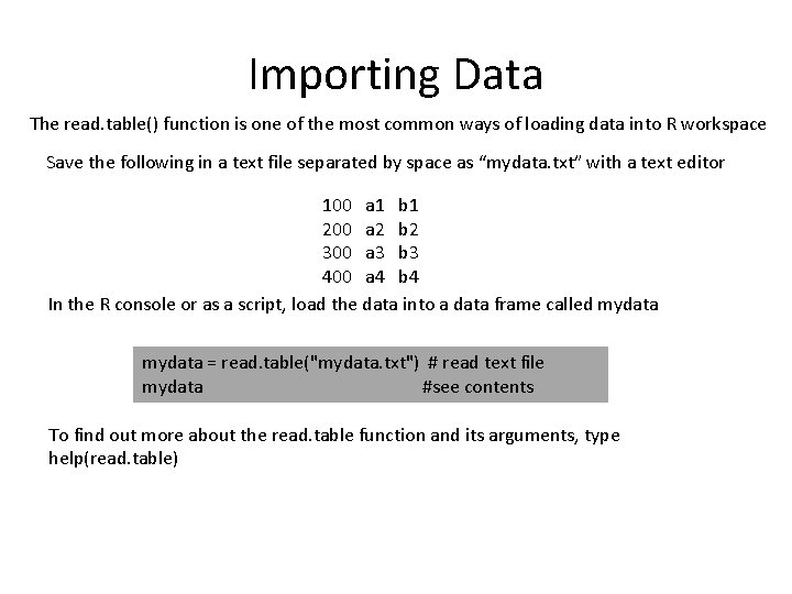
Importing Data The read. table() function is one of the most common ways of loading data into R workspace Save the following in a text file separated by space as “mydata. txt” with a text editor 100 a 1 b 1 200 a 2 b 2 300 a 3 b 3 400 a 4 b 4 In the R console or as a script, load the data into a data frame called mydata = read. table("mydata. txt") # read text file mydata #see contents To find out more about the read. table function and its arguments, type help(read. table)

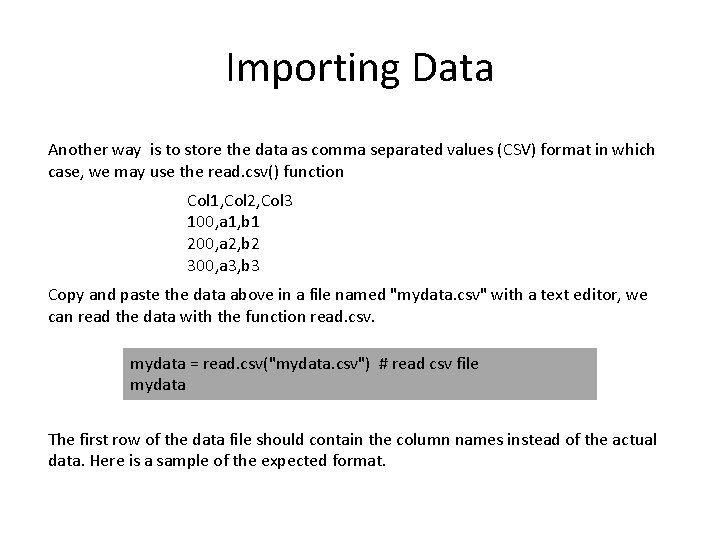
Importing Data Another way is to store the data as comma separated values (CSV) format in which case, we may use the read. csv() function Col 1, Col 2, Col 3 100, a 1, b 1 200, a 2, b 2 300, a 3, b 3 Copy and paste the data above in a file named "mydata. csv" with a text editor, we can read the data with the function read. csv. mydata = read. csv("mydata. csv") # read csv file mydata The first row of the data file should contain the column names instead of the actual data. Here is a sample of the expected format.

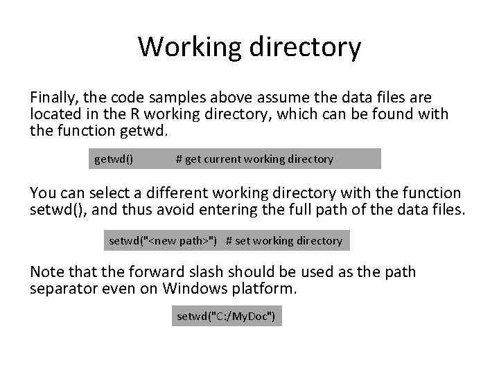
Working directory Finally, the code samples above assume the data files are located in the R working directory, which can be found with the function getwd() # get current working directory You can select a different working directory with the function setwd(), and thus avoid entering the full path of the data files. setwd("<new path>") # set working directory Note that the forward slash should be used as the path separator even on Windows platform. setwd("C: /My. Doc")

Special programmatic elements

%in% Special programmatic elements Special values Apply

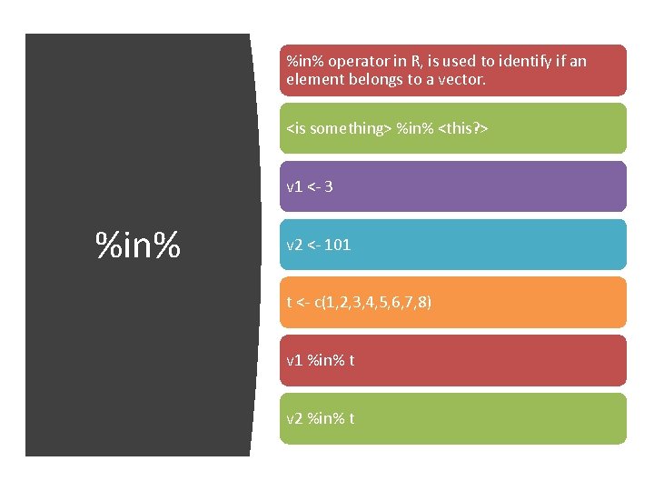
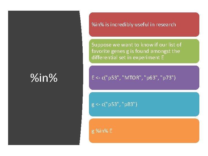
%in% operator in R, is used to identify if an element belongs to a vector. <is something> %in% <this? > v 1 <- 3 %in% v 2 <- 101 t <- c(1, 2, 3, 4, 5, 6, 7, 8) v 1 %in% t v 2 %in% t

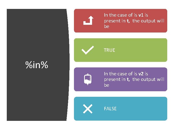
In the case of is v 1 is present in t, the output will be TRUE %in% In the case of is v 2 is present in t, the output will be FALSE

%in% is incredibly useful in research Suppose we want to know if our list of favorite genes g is found amongst the differential set in experiment E %in% E <- c("p 53", "MTOR", "p 63", "p 73") g <- c("p 53", "p 83") g %in% E

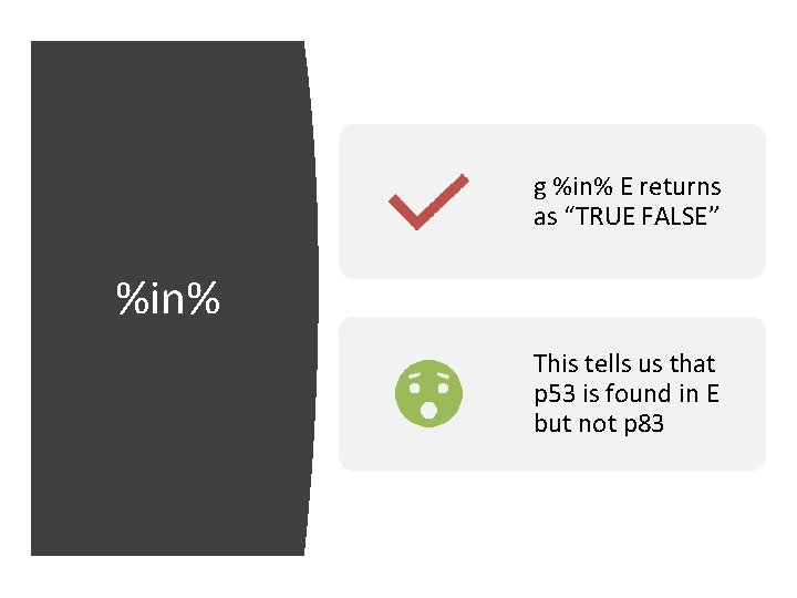
g %in% E returns as “TRUE FALSE” %in% This tells us that p 53 is found in E but not p 83

NA (Missing data) Special values Na. N (Not a Number) Inf (Infinite)

Special values

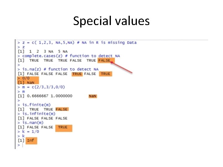
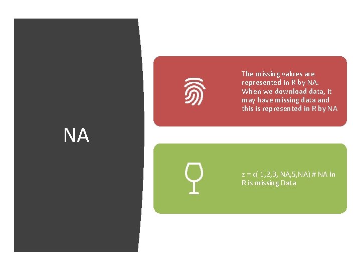
The missing values are represented in R by NA. When we download data, it may have missing data and this is represented in R by NA NA z = c( 1, 2, 3, NA, 5, NA) # NA in R is missing Data

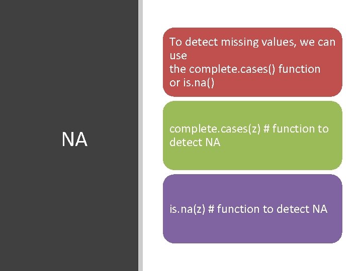
To detect missing values, we can use the complete. cases() function or is. na() NA complete. cases(z) # function to detect NA is. na(z) # function to detect NA

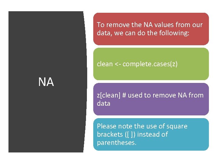
To remove the NA values from our data, we can do the following: clean <- complete. cases(z) NA z[clean] # used to remove NA from data Please note the use of square brackets ([ ]) instead of parentheses.

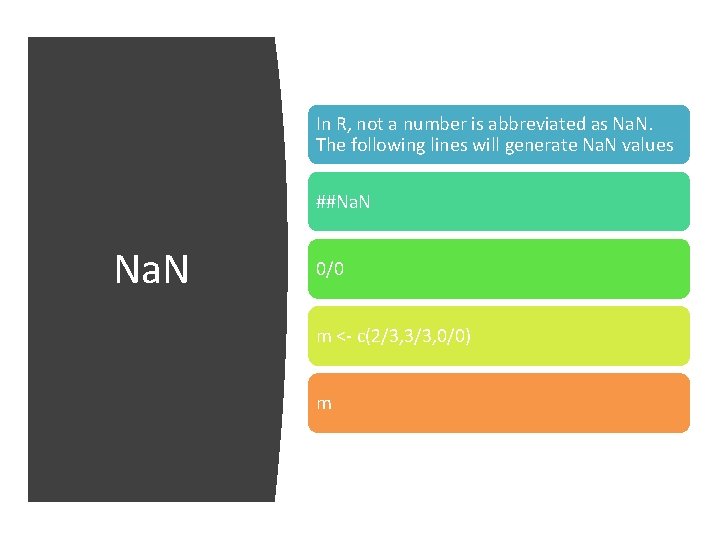
In R, not a number is abbreviated as Na. N. The following lines will generate Na. N values ##Na. N 0/0 m <- c(2/3, 3/3, 0/0) m

The is. finite(), is. infinite(), or is. nan functions will generate logical values (TRUE or FALSE). is. finite(m) Na. N is. infinite(m) is. nan(m)

The following line will generate inf as a special value in R Inf ## infinite k = 1/0

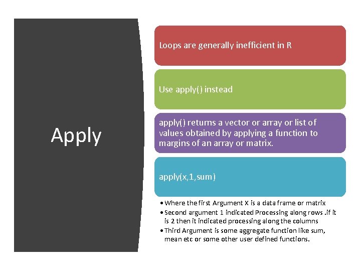
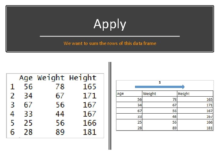
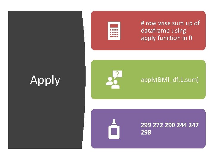
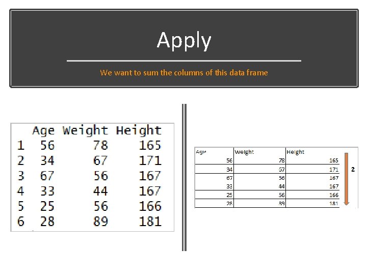
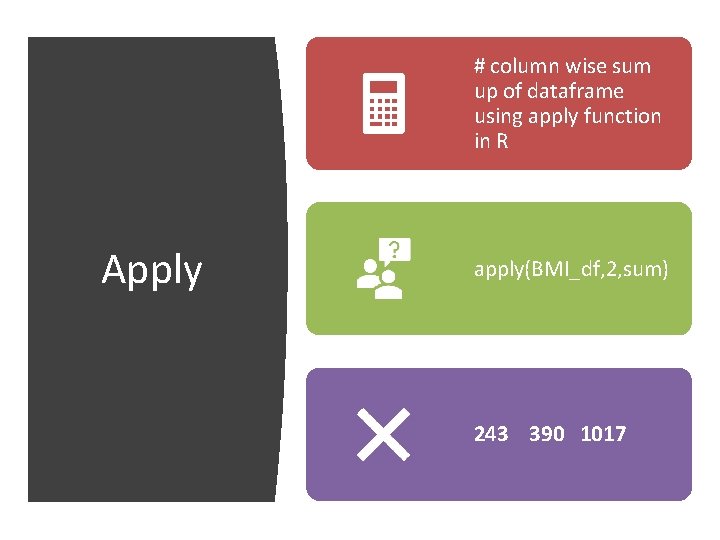
Loops are generally inefficient in R Use apply() instead Apply apply() returns a vector or array or list of values obtained by applying a function to margins of an array or matrix. apply(x, 1, sum) • Where the first Argument X is a data frame or matrix • Second argument 1 indicated Processing along rows. if it is 2 then it indicated processing along the columns • Third Argument is some aggregate function like sum, mean etc or some other user defined functions.

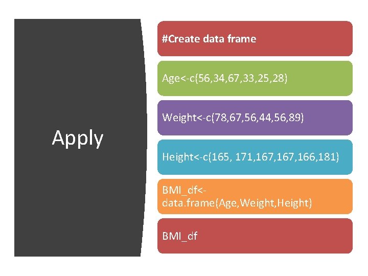
#Create data frame Age<-c(56, 34, 67, 33, 25, 28) Apply Weight<-c(78, 67, 56, 44, 56, 89) Height<-c(165, 171, 167, 166, 181) BMI_df<data. frame(Age, Weight, Height) BMI_df

Apply We want to sum the rows of this data frame

# row wise sum up of dataframe using apply function in R Apply apply(BMI_df, 1, sum) 299 272 290 244 247 298

Apply We want to sum the columns of this data frame

# column wise sum up of dataframe using apply function in R Apply apply(BMI_df, 2, sum) 243 390 1017

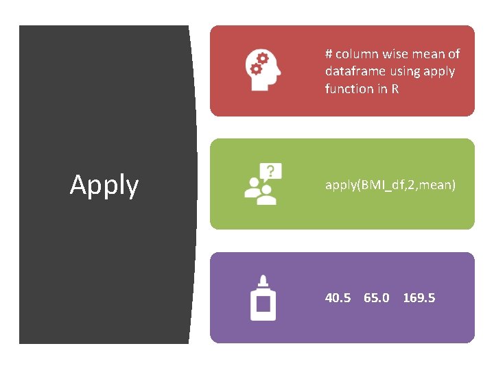
# column wise mean of dataframe using apply function in R Apply apply(BMI_df, 2, mean) 40. 5 65. 0 169. 5

END OF SEGMENT Let’s take a break