269202 ALGORITHMS FOR ISNE DR KENNETH COSH WEEK

269202 ALGORITHMS FOR ISNE DR. KENNETH COSH WEEK 7

REVIEW Multiway Trees B-Trees B*Trees B+Trees Bit Trees Tries

THIS WEEK This week we introduce graphs; a data structure with more flexibility than the hierarchical data structure. a data structure with less limitations, i. e. where parent / child nodes aren’t necessary Graphs are versatile data structures which represent a large number of situations in a large variety of domains. Essentially graphs are a collection of vertices (or nodes), and connections between them (or edges).

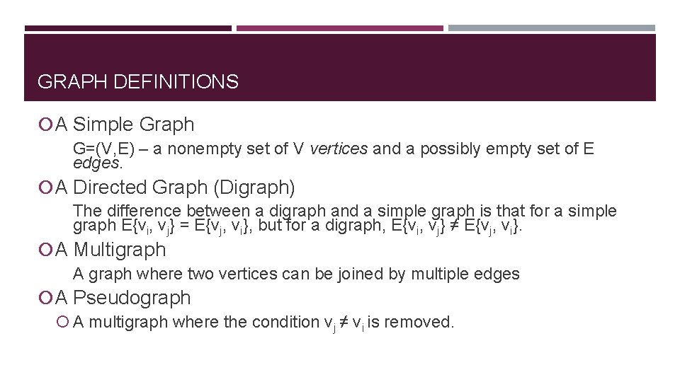
GRAPH DEFINITIONS A Simple Graph G=(V, E) – a nonempty set of V vertices and a possibly empty set of E edges. A Directed Graph (Digraph) The difference between a digraph and a simple graph is that for a simple graph E{vi, vj} = E{vj, vi}, but for a digraph, E{vi, vj} ≠ E{vj, vi}. A Multigraph A graph where two vertices can be joined by multiple edges A Pseudograph A multigraph where the condition vj ≠ vi is removed.

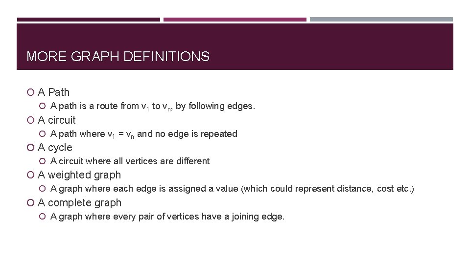
MORE GRAPH DEFINITIONS A Path A path is a route from v 1 to vn, by following edges. A circuit A path where v 1 = vn and no edge is repeated A cycle A circuit where all vertices are different A weighted graph A graph where each edge is assigned a value (which could represent distance, cost etc. ) A complete graph A graph where every pair of vertices have a joining edge.

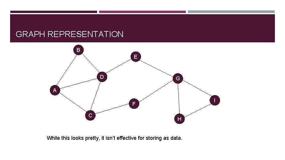
GRAPH REPRESENTATION B E D G A I F C H While this looks pretty, it isn’t effective for storing as data.

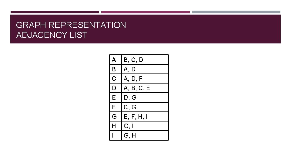
GRAPH REPRESENTATION ADJACENCY LIST A B, C, D. B A, D C A, D, F D A, B, C, E E D, G F C, G G E, F, H, I H G, I I G, H

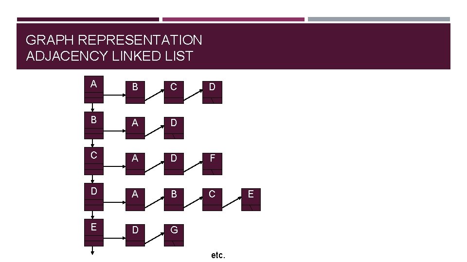
GRAPH REPRESENTATION ADJACENCY LINKED LIST A B C B A D C A D F D A B C E D G D etc. E

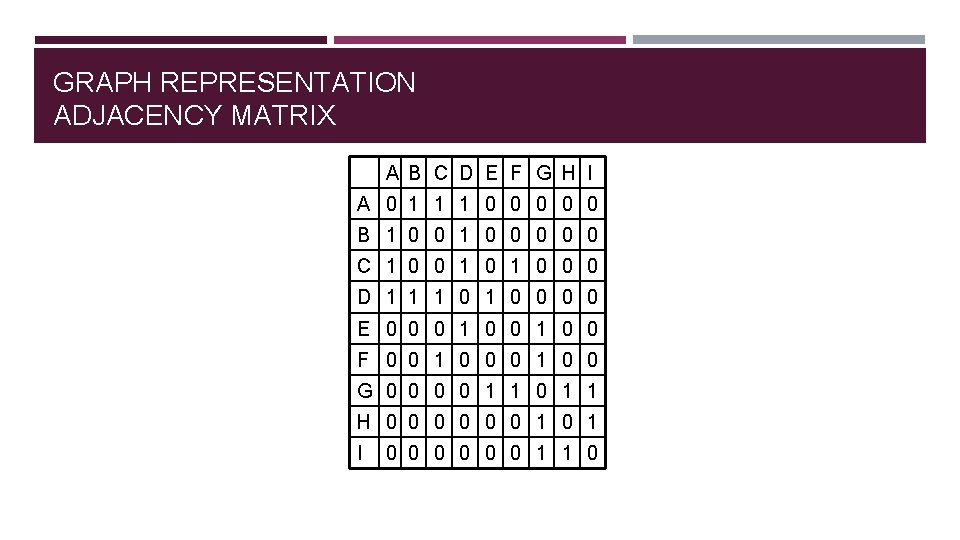
GRAPH REPRESENTATION ADJACENCY MATRIX A B C D E F G H I A 0 1 1 1 0 0 0 B 1 0 0 0 0 0 C 1 0 0 0 D 1 1 1 0 0 0 0 E 0 0 0 1 0 0 F 0 0 1 0 0 G 0 0 1 1 H 0 0 0 1 0 1 I 0 0 0 1 1 0

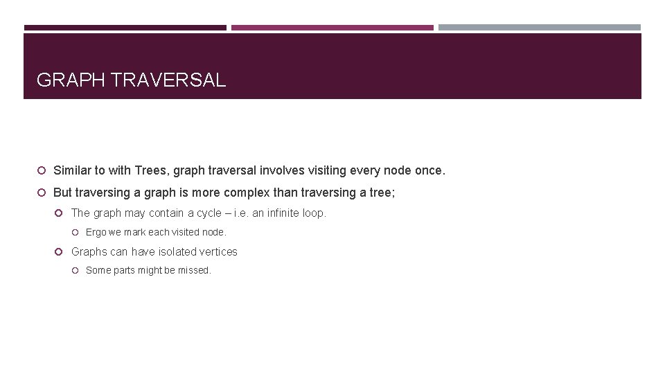
GRAPH TRAVERSAL Similar to with Trees, graph traversal involves visiting every node once. But traversing a graph is more complex than traversing a tree; The graph may contain a cycle – i. e. an infinite loop. Ergo we mark each visited node. Graphs can have isolated vertices Some parts might be missed.

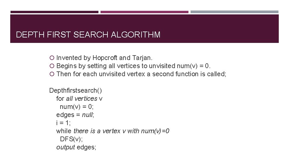
DEPTH FIRST SEARCH ALGORITHM Invented by Hopcroft and Tarjan. Begins by setting all vertices to unvisited num(v) = 0. Then for each unvisited vertex a second function is called; Depthfirstsearch() for all vertices v num(v) = 0; edges = null; i = 1; while there is a vertex v with num(v)=0 DFS(v); output edges;

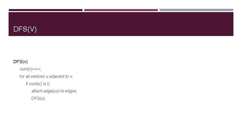
DFS(V) DFS(v) num(v)=i++; for all vertices u adjacent to v; if num(u) is 0; attach edge(uv) to edges; DFS(u);

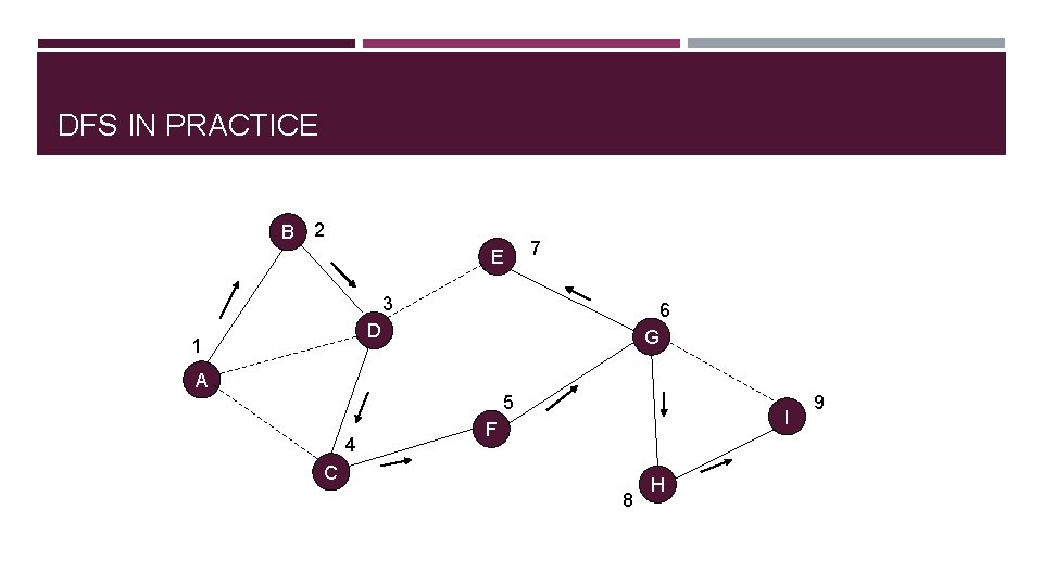
DFS IN PRACTICE B 2 E 7 3 6 D 1 G A 5 4 I F C 8 H 9

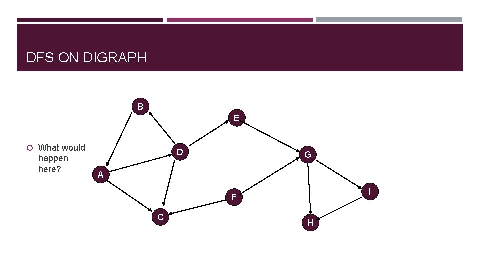
DFS ON DIGRAPH B E What would happen here? D G A I F C H

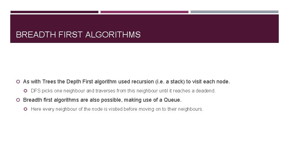
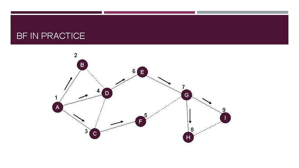
BREADTH FIRST ALGORITHMS As with Trees the Depth First algorithm used recursion (i. e. a stack) to visit each node. DFS picks one neighbour and traverses from this neighbour until it reaches a deadend. Breadth first algorithms are also possible, making use of a Queue. Here every neighbour of the node is visited before moving on to their neighbours.

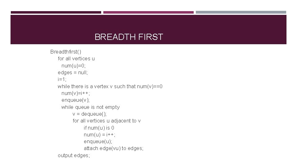
BREADTH FIRST Breadthfirst() for all vertices u num(u)=0; edges = null; i=1; while there is a vertex v such that num(v)==0 num(v)=i++; enqueue(v); while queue is not empty v = dequeue(); for all vertices u adjacent to v if num(u) is 0 num(u) = i++; enqueue(u); attach edge(vu) to edges; output edges;

BF IN PRACTICE 2 B 6 E 7 G 4 D 1 A F 3 C 9 I 5 8 H

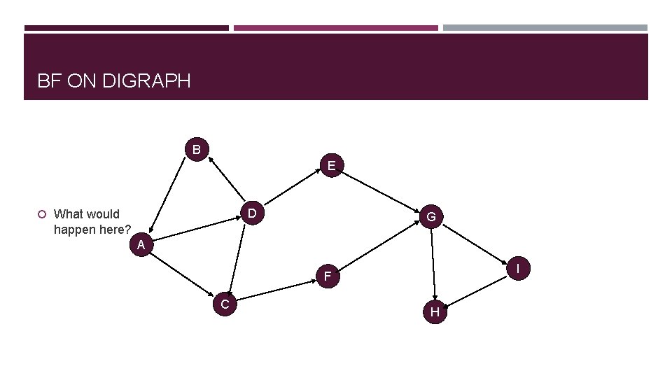
BF ON DIGRAPH B E D What would G happen here? A I F C H

BF VS DFS EFFICIENCY The complexity of each version depends partly on how the data about the graph is stored, whether in an adjacency list or an adjacency matrix. It also depends on how many isolated edges there are; This influences the number of outer loops. Worst case when every node is isolated.

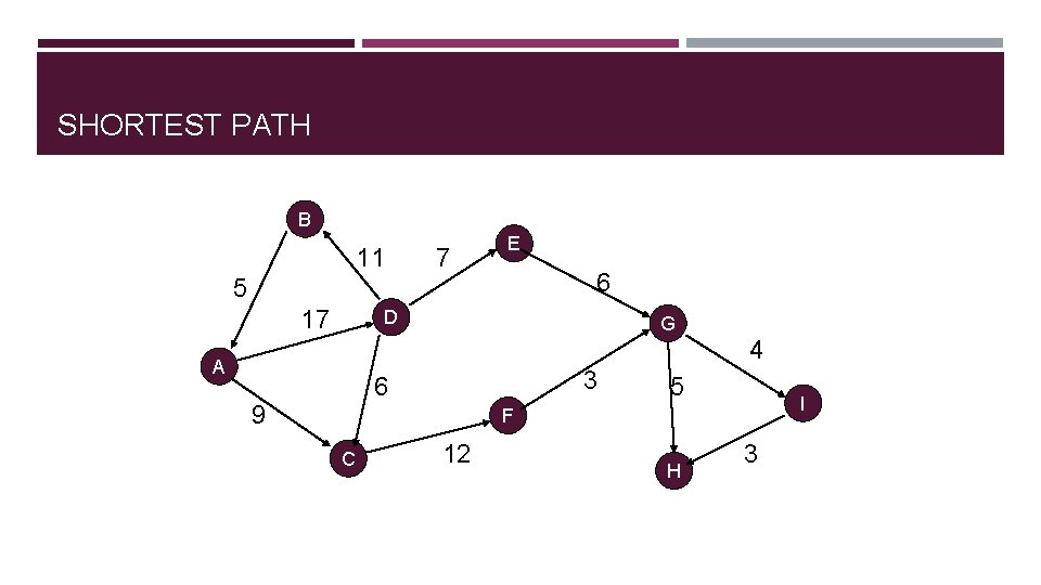
SHORTEST PATH Finding the shortest path between nodes is a classic Graph theory problem One we have mentioned already. Shortest path could be used to design delivery routes, to calculate data transmission costs etc. Each edge is assigned a value, and the shortest path is the path with the least value.

SHORTEST PATH B 11 7 E 6 5 17 D G 4 A 3 6 9 5 I F C 12 H 3

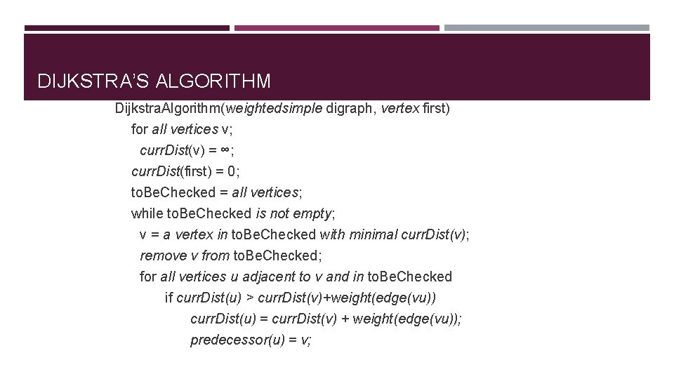
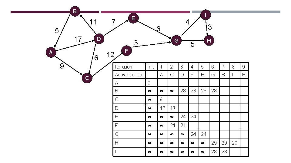
DIJKSTRA’S ALGORITHM Dijkstra. Algorithm(weightedsimple digraph, vertex first) for all vertices v; curr. Dist(v) = ∞; curr. Dist(first) = 0; to. Be. Checked = all vertices; while to. Be. Checked is not empty; v = a vertex in to. Be. Checked with minimal curr. Dist(v); remove v from to. Be. Checked; for all vertices u adjacent to v and in to. Be. Checked if curr. Dist(u) > curr. Dist(v)+weight(edge(vu)) curr. Dist(u) = curr. Dist(v) + weight(edge(vu)); predecessor(u) = v;

DIJKSTRA’S ALGORITHM COMMENTRY First all nodes are added to a list of ‘to. Be. Checked’. They are all assigned an infinite curr. Dist(v), except the start node, who’s distance is 0. Each node is tested in turn – starting with close by nodes – and for each we see if they provide a quicker route to their neighbours than has been found before.

B 11 I E 7 6 5 17 D A 6 9 DIJKSTRA IN PRACTICE G 3 12 init Active vertex 3 H 5 F Iteration C 4 1 2 3 4 5 6 7 8 9 A C D F E G B I H ∞ 28 28 24 29 A 0 B ∞ ∞ C ∞ 9 D ∞ 17 17 E ∞ ∞ ∞ 24 F ∞ ∞ 21 21 G ∞ ∞ 24 24 H ∞ ∞ ∞ 29 29 I ∞ ∞ ∞ 28 28

DIJKSTRA’S PROBLEM Dijkstra does have a problem, in that it doesn’t work if there are negative valued edges. For a graph with negative weights, the entire graph would need to be processed before distances can be confirmed.

ALL-TO-ALL SHORTEST PATHS So far we have dealt with the situation where there is a single start point, and we calculate the distance to each other node from there. How about if we wanted to calculate the shortest path from any node to any other node? Surprisingly the code for this is simple, even if it is computationally complex.

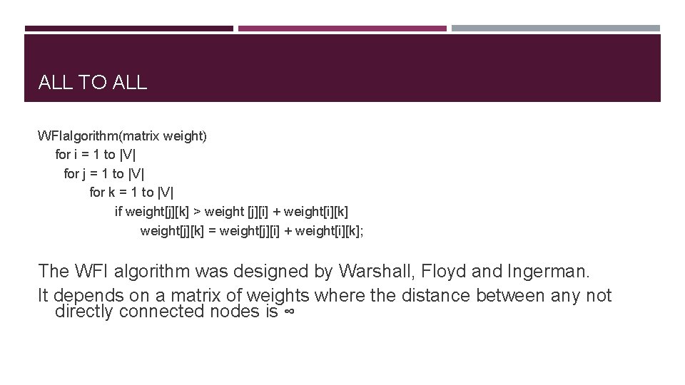
ALL TO ALL WFIalgorithm(matrix weight) for i = 1 to |V| for j = 1 to |V| for k = 1 to |V| if weight[j][k] > weight [j][i] + weight[i][k] weight[j][k] = weight[j][i] + weight[i][k]; The WFI algorithm was designed by Warshall, Floyd and Ingerman. It depends on a matrix of weights where the distance between any not directly connected nodes is ∞

ALL TO ALL See if you can work out how it works. What is Big-O for this algorithm?

SUB PROBLEMS One possible useful side effect of the WFI algorithm is that cycles can be detected. But the WFI algorithm isn’t efficient enough at detecting cycles for many cases. Next we will briefly investigate two smaller problems, which commonly feature in larger graphing problems Cycle Detection Union Find

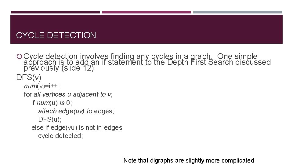
CYCLE DETECTION Cycle detection involves finding any cycles in a graph. One simple approach is to add an if statement to the Depth First Search discussed previously (slide 12) DFS(v) num(v)=i++; for all vertices u adjacent to v; if num(u) is 0; attach edge(uv) to edges; DFS(u); else if edge(vu) is not in edges cycle detected; Note that digraphs are slightly more complicated

UNION FIND The union-find algorithm first ‘finds’ which set an element is in, and second ‘unions’ two sets together. It is a problem found when dealing with disjoint sets. For our purposes it can be used to determine if two nodes are connected in a graph. The next problem will suggest an application for Union Find. For now the function union(x, y) where x and y are nodes, first tests if they are in the same set, and then merges them together, into a linked list.

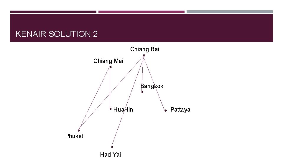
KENAIR’S PROBLEM Suppose I’m running an airline which flies connections between the following cities; Bangkok, Chiang Mai, Chiang Rai, Phuket, Hua Hin, Pattaya & Had Yai. Sadly my airline has fallen on hard times, so I have to reduce the number of routes. My challenge is to enable people to still be able to connect to all destinations only using Ken. Air – even if they have to make multiple connections.

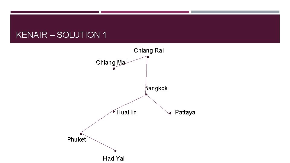
KENAIR – SOLUTION 1 Chiang Rai Chiang Mai Bangkok Hua. Hin Phuket Had Yai Pattaya

KENAIR SOLUTION 2 Chiang Rai Chiang Mai Bangkok Hua. Hin Phuket Had Yai Pattaya

KENAIR So which is better? Clearly it will depend on the cost of flying each route – ideally we want to keep the cheapest routes open, and close the more expensive ones. Each map is known as a ‘Spanning Tree’, in this task we want to find the minimum spanning tree

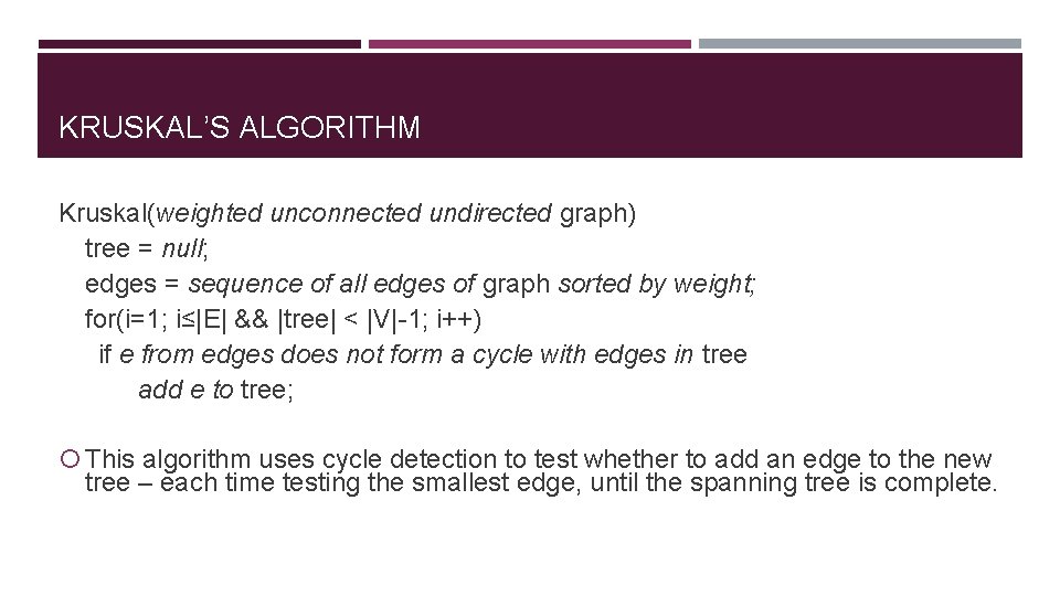
KRUSKAL’S ALGORITHM Kruskal(weighted unconnected undirected graph) tree = null; edges = sequence of all edges of graph sorted by weight; for(i=1; i≤|E| && |tree| < |V|-1; i++) if e from edges does not form a cycle with edges in tree add e to tree; This algorithm uses cycle detection to test whether to add an edge to the new tree – each time testing the smallest edge, until the spanning tree is complete.

TOPOLOGICAL SORT Many graphs, specifically digraphs, represent tasks to be performed in a particular order; a process diagram the course pre-requisites diagram In this case a Topological Sort will order the nodes in the graph; Locate the root node – 269101. Locate the next node.

TOPOLOGICAL SORT PSEUDOCODE toposort(digraph) for i = 1 to |V| find minimal vertex v; num(v) = i; remove v from digraph and all edges; Try this out on the course outline.

NETWORKS A network is a special type of graph. A network is a digraph. The digraph has one source vertex with no incoming edges. The digraph has one sink vertex with no outgoing edges. Each edge has a capacity. A network can be used to model many situations, such as water flowing through some pumps and pipes, or data moving through a computer network.

PROGRAMMING ASSIGNMENT Or rather Pseudocoding assignment A key algorithm when dealing with networks is to calculate the maximal flow through it. Part 1: Write Pseudocode which calculates the maximal flow through a network. Demonstrate your algorithm using a sample network.

PROGRAMMING ASSIGNMENT Pseudocoding The capacity of an edge is only one factor, other factors may influence the cost of transferring units along edges. Therefore each edge should contain a cost parameter as well as a capacity parameter. Part 2: A further important algorithm designs how to flow items through a network. If there is 1 item what route should it take, if there are ‘n’ items which routes should they take. Consider an algorithm to deal with this.

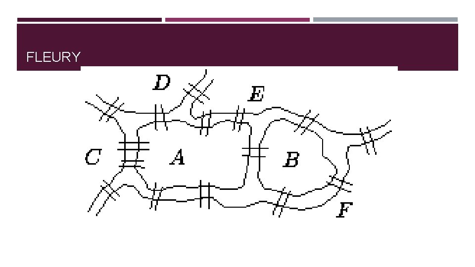
EULERIAN GRAPHS An Eulerian Trail is a route through a graph which includes every edge only once. An Eulerian Cycle is an Eulerian Trail which is also a cycle. An Eulerian Graph is a graph containing an Eulerian Cycle.

EULERIAN GRAPHS A graph is Eulerian if every vertex is incident to an even number of edges. Prove this! A graph contains an Eulerian Trail if it has exactly two vertices incident with an odd number of edges.

FLEURY

THE CHINESE POSTMAN A Chinese postman picks up his letters from the post office and then delivers them to a certain area before returning to the post office. His walk should be a short as possible, but he needs to traverse every street at least once.

THE CHINESE POSTMAN Is the graph Eulerian? If the graph is Eulerian, then finding any Eulerian cycle will solve the problem. If the graph isn’t Eulerian, how can we make it Eulerian? For any pair of nodes with an odd number of incident edges, we can repeat the edge. Repeat edges until there are no nodes with odd numbers of incident edges to produce an Eulerian graph. Clearly here we need to try to choose the shortest edges to repeat.

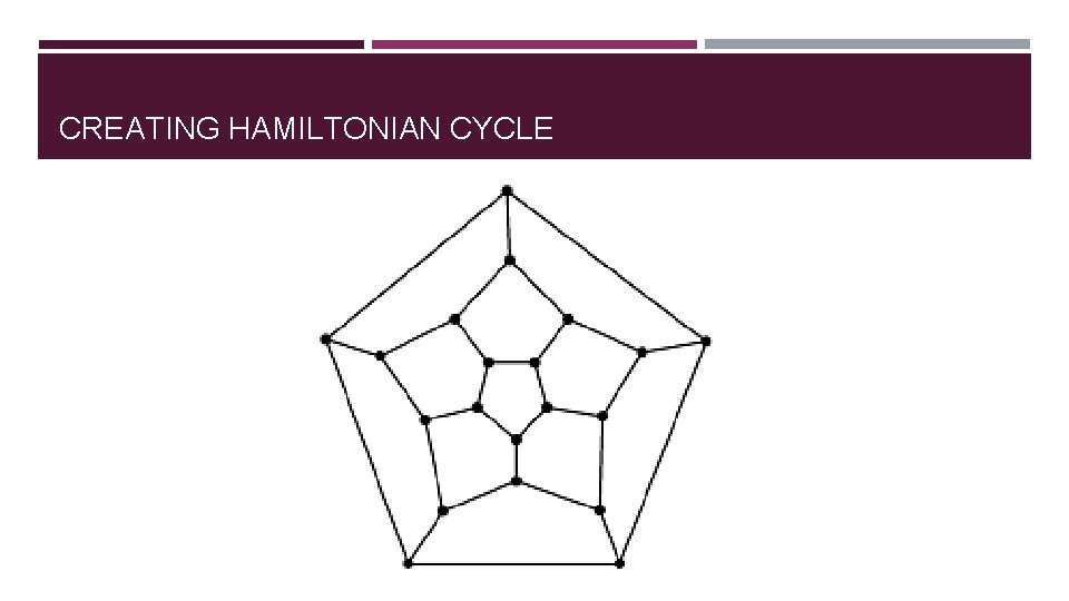
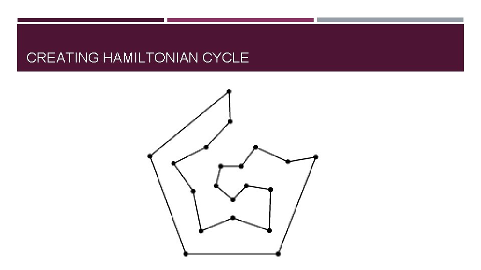
HAMILTONIAN GRAPHS A Hamiltonian cycle in a graph is a cycle which passes through all the vertices of the graph. A Hamilton Graph is a graph where at least one Hamiltonian cycle exists. All complete graphs are hamiltonian.

FINDING A HAMILTONIAN CYCLE In some problems (see TSP), it is allowed to remove some edges in order to create a Hamiltonian Graph. i. e. we can begin with a complete graph, and then remove edges to find a Hamiltonian cycle. Another approach is to begin from a minimum spanning tree – which is similar to a hamiltonian cycle with one edge removed. The sum of the edges in the minimum spanning tree must be less than the minimum tour of a hamiltonian cycle.

CREATING HAMILTONIAN CYCLE

CREATING HAMILTONIAN CYCLE

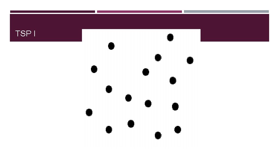
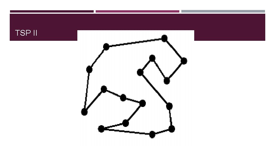
THE TRAVELLING SALESMAN The travelling salesman problem is widely touted – and is a popular NP-Complete problem. A salesman has to visit every city, and he must take the shortest route between each. Clearly this problem is finding the shortest Hamiltonian cycle. While the previous slide illustrated a hamiltonian cycle, it may not have been the shortest hamiltonian cycle.

TSP I

TSP II

SOLVING TSP (APPROACH 1) Obviously the TSP problem is considered NP-Complete. But there are several ‘unsatisfactory’ solutions available. One approach is to take a minimum spanning tree and then join the two ‘end’ nodes. Consider the minimum spanning trees we looked at before, one had 3 ends, and the other had 4 ends!

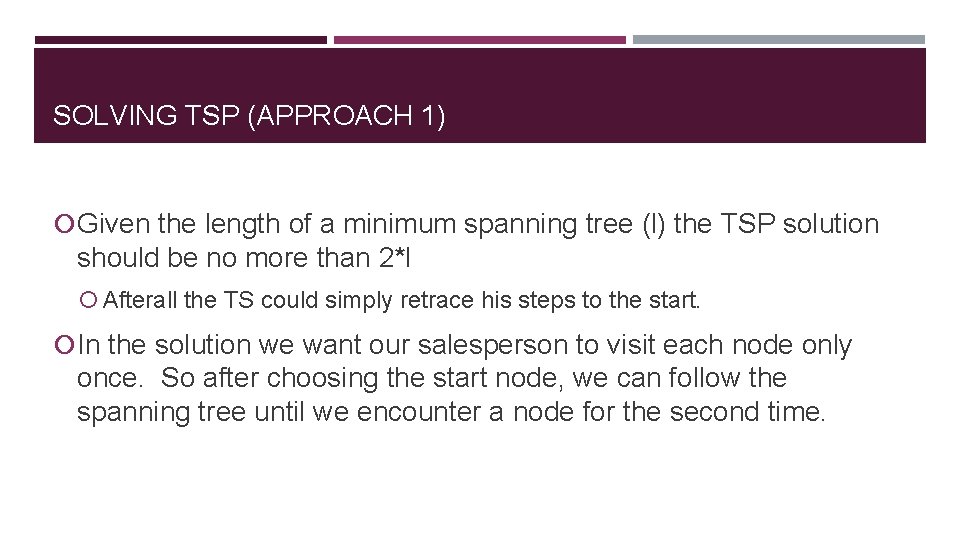
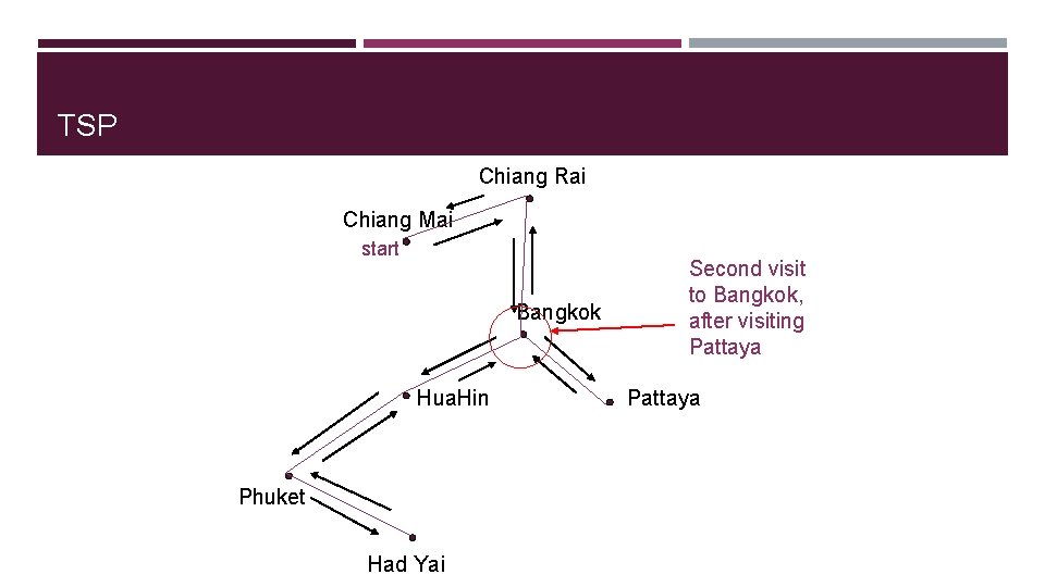
SOLVING TSP (APPROACH 1) Given the length of a minimum spanning tree (l) the TSP solution should be no more than 2*l Afterall the TS could simply retrace his steps to the start. In the solution we want our salesperson to visit each node only once. So after choosing the start node, we can follow the spanning tree until we encounter a node for the second time.

TSP Chiang Rai Chiang Mai start Bangkok Hua. Hin Phuket Had Yai Second visit to Bangkok, after visiting Pattaya

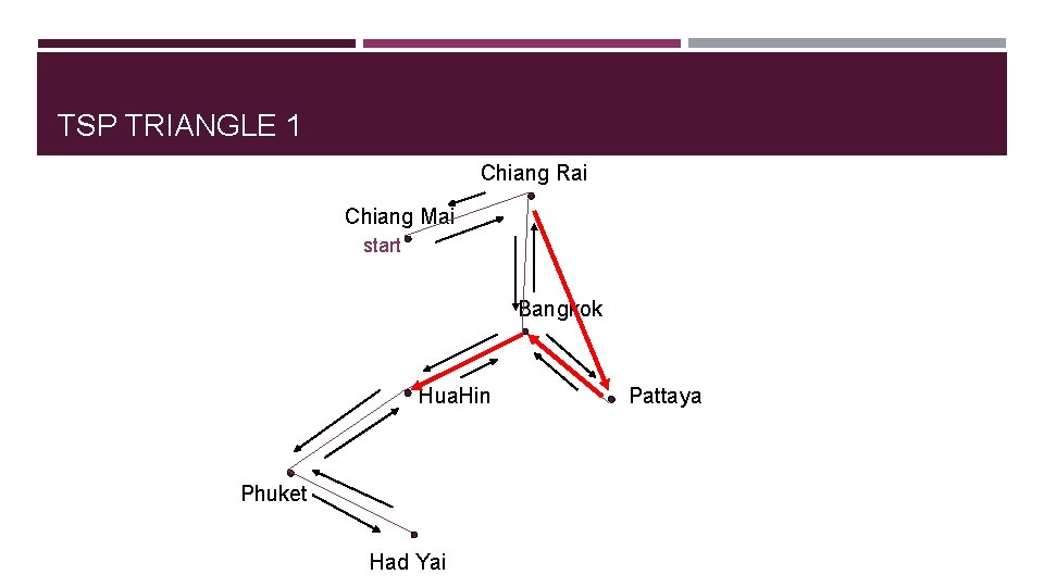
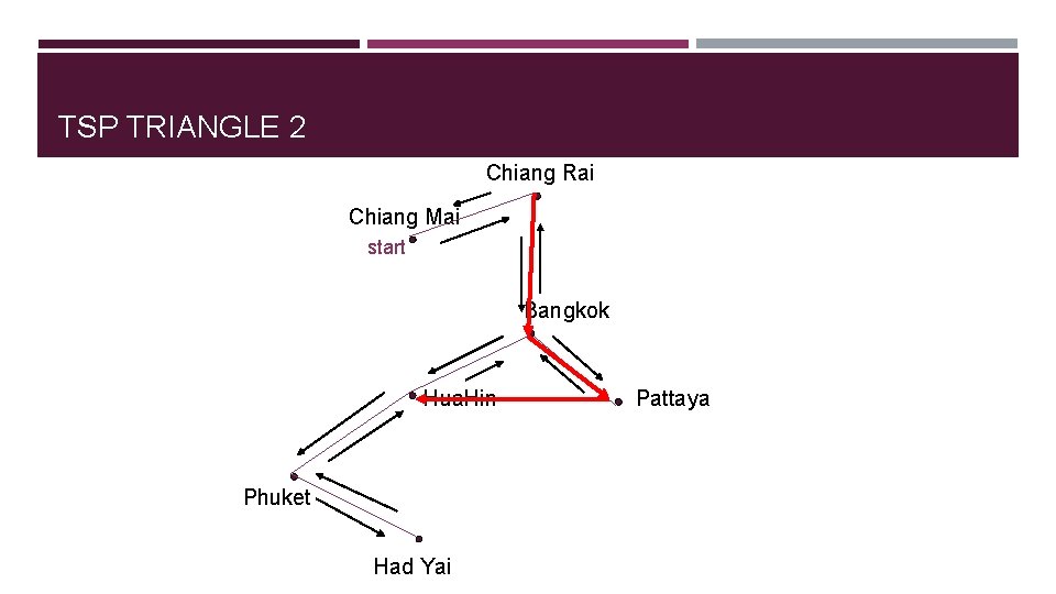
TRIANGLES We know that the length of the longest side of a triangle is shorter than the sum of the other two sides. Taking this we can use one of two alternative triangles to avoid the second visit. Choosing which of course depends on their respective lengths.

TSP TRIANGLE 1 Chiang Rai Chiang Mai start Bangkok Hua. Hin Phuket Had Yai Pattaya

TSP TRIANGLE 2 Chiang Rai Chiang Mai start Bangkok Hua. Hin Phuket Had Yai Pattaya

TSP CONTINUES The travelling salesman can then continue along his route, until the second time he revisits a node; Returning to Phuket after Had. Yai. What happens next?

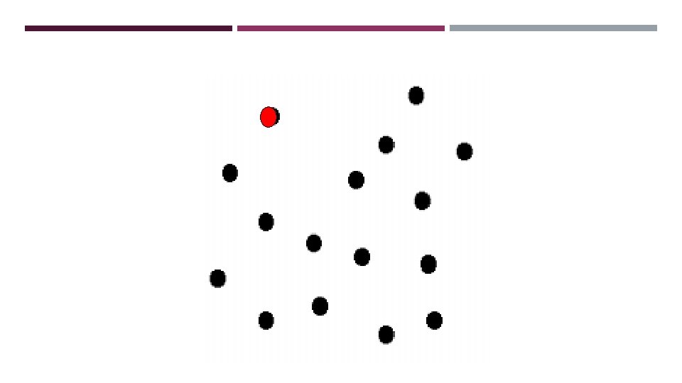
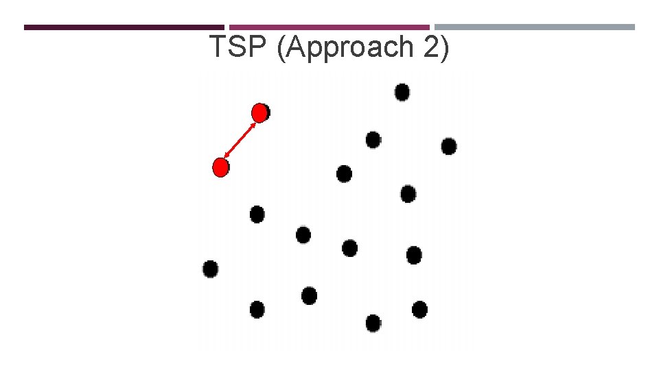
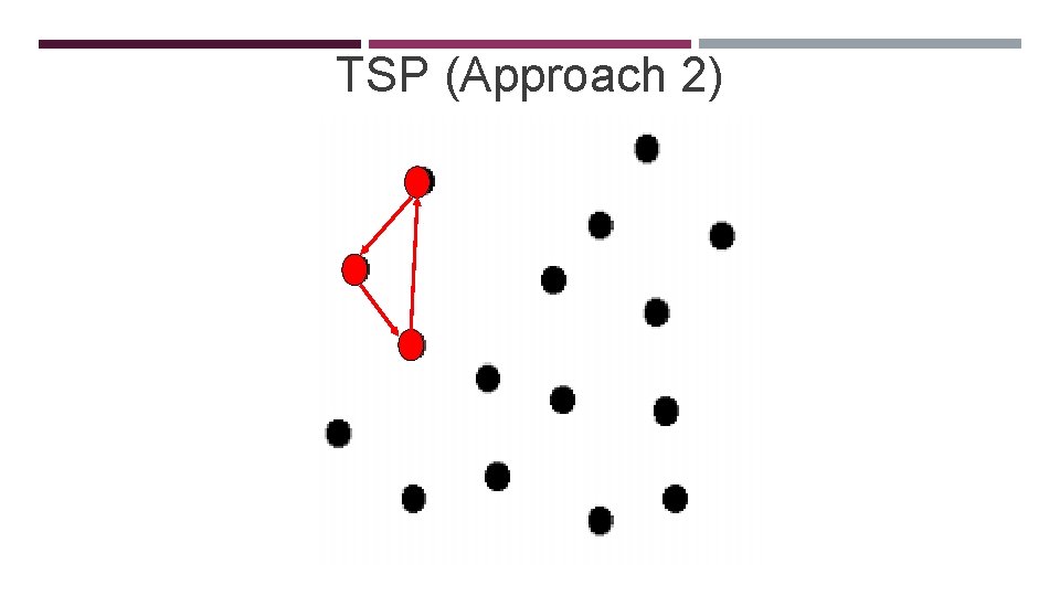
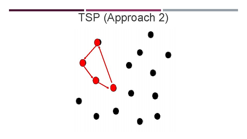
SOLVING TSP (APPROACH 2) A second approach takes a root node, and then inserts its nearest neighbour to create a loop. Then the next nearest neighbour is added, normally creating a triangle. Then the next nearest neighbour is added to link to its 2 closest neighbours. Etc. until all nodes are linked.

TSP (APPROACH 2)

TSP (Approach 2)

TSP (Approach 2)

TSP (Approach 2)