Transcriptomics towards RNASeq Federico M Giorgi federico giorgigmail

Transcriptomics – towards RNASeq Federico M. Giorgi – federico. giorgi@gmail. com Analisi del Genoma e Bioinformatica Corso di Laurea Specialistica in Biotecnologie delle piante e degli animali

Overview of the course Transcription and Transcriptomics Day 1 23/04/2012 Room β 3 Transcriptomics methods: Microarrays Exercises on Microarray analysis Day 2 02/05/2012 Room 35 Day 3 07/05/2012 Room β 3 RNASeq Real cases – Further applications RNASeq exercises

Background - Transcriptomics Transcriptome is the complete set of transcripts in a cell, and their quantity, for a specific developmental stage or physiological condition.

Background - Transcriptomics is the study of the Transcriptome Key Aims of Trascriptomics: • To catalogue all species of transcript • To determine the transcriptional structure(s) of genes • To quantify the changing expression levels of each transcript during development and under different conditions. Final goals: • To monitor molecular responses to treatments • To understand how the cell functions

Transcriptomics network Transcripts interact with each other, and with proteins, lipids, metabolites. . . Some m. RNAs get translated into Transcription Factors, which control the expression of other transcripts. . . A representation of these relationships is usually a complex NETWORK

Transcriptomics techniques Hybridization-based Northern Blot • • • Requires prior knowledge of the organism, for probe design The first method for specific RNA detection Based initially on radioactive probes Not fully quantitative Low yield Still required sometimes as validation for more modern techniques • Can cover almost an entire transcriptome Microarrays • Exon arrays can detect specific splice variants • Tiling arrays can detect inter-genic regions • Still less expensive than high-throughput sequencing (NGS) • Problems with cross-hybridizing probes

Transcriptomics techniques Real Time Quantitative PCR Requires prior knowledge of the organism, for primers design (but degenerated primers can be used) • Calculates the Ct (PCR cycle at which the specific transcript appears above a detection threshold) • Normalizes the Ct versus two or more housekeeping genes – usually constant in their expression across tissues (e. g. Tubulin or EF 1α in Arabidopsis thaliana) • Can be efficiently used for up to 100 transcripts. And it’s considered the golden standard for single-gene papers

Transcriptomics techniques Sequence-based Sanger • • Long sequences (1500 nt) Low throughput Expensive Very rarely used for transcriptome Tag-based • • SAGE, CAGE, MPSS Higher throughput Expensive Mapping problems RNASeq • • High throughput Wide Transcriptome Fully quantitative High information/cost ratio • Doesn’t require prior knowledge of the organism: everything is sequenced. . . Even contaminants • Requires a consistent bioinformatics infrastructure • Required specific and fast software to be dealt with

Microarray classes Double channel Single Channel Two samples are tagged with a green (Cy 3) or a red (Cy 5) chromophore, and then compared at the same time on the chip Normalization is achieved within the array itself, e. g. (Affymetrix) by the presence of Mismatch probes paired with Perfect Match probes Non. Affymetrix Agilent Nimblegen Custom spotting Affymetrix

Affymetrix Microarrays Total m. RNA AAAA c. DNA Reverse transcription Biotin-labeled c. RNA In vitro transcription B B AAAA B B Fragmentation B B B Gene. Chip Expression array B B Hybridization Wash and stain B Scan and quantitate Data processing

Affymetrix Microarrays • A chip consists in a number of probesets • Probesets are intended to measure expression for a specific m. RNA/gene (or family of genes) • Probesets consist of a collection of 25 mer probes selected from the target sequence

Microarray Probes Gene -m. RNA 22810 genes (probesets)* “Perfect match” probeset (~ 11 probes per gene) “Mismatch” probeset (to detect unspecific signal) * Affymetrix ATH 1 Arabidopsis Gene. Chip©

Microarray Probes

Microarray – Data processing Raw optical image (DAT file) Raw intensity values (CEL file)

Microarray – Data processing Summarizes 11 probes’ values in 1 gene value Background subtraction Raw intensity values (CEL file) Normalization Makes arrays comparable Summarization

Preprocessing: RMA and MAS 5 RMA background model Quantile Median polish (multi-array) Background correction Normalization Summarization Scale Tukey biweight robust median (single-array) Zone effect MAS 5 Subtraction of mismatch probes

Which one works better? • RMA/GCRMA is ecellent for differential expression (see Cope et al. 2004 benchmark) • MAS 5, by keeping arrays separated, is good for other tasks that require independence of measurements, e. g. Gene Network Reconstruction (Lim et al. , 2007)

Other less known (and never used) microarray preprocessing methods • d. Chip (Li-Wong, 2001) • FARMS (Hochreiter, 2006; performs better than all methods in benchmark studies; it’s also very fast, but nobody uses it) • PLIER (new Affymetrix standard, recent winner in a comparison with RT-PCR measurements – Gyorffy et al. , 2009) • t. RMA (Giorgi et al. , 2010; fixes problems in multimatching probesets, a common issue with microarray data)

Microarray Probes Gene -m. RNA 22810 genes (probesets)* “Perfect match” probeset (~ 11 probes per gene) “Mismatch” probeset (to detect unspecific signal) * Affymetrix ATH 1 Arabidopsis Gene. Chip©

Probesets mapping to Arabidopsis genes 0 mismatches BLAST bitscore >=50. 1 25/25 alignment 0 mismatches

Probesets mapping to Arabidopsis genes 1 mismatch BLAST bitscore >=42. 1 21/25 alignment 1 mismatch

Probesets mapping to Arabidopsis genes 2 mismatches Probes with 2 mismatches detect a m. RNA with a signal only 20% smaller than a 0 mismatches probe (Hooyberghs et al. , 2009) BLAST bitscore >=34. 2 17/25 alignment 2 mismatches

Microarrays vs. RNASeq Count vs. continuous

Microarrays vs. RNASeq Signal vs. Quantity plots Saturation Microarray signal Limit of detection Real quantity of transcript

Microarrays vs. RNASeq Gene length bias Tarazona 2011

Exercises I see and I forget I read and I remember I do and I understand Confucius 551 B. C. – 479 B. C.

Exercise – get some microarrays Google for: Gene Expression Omnibus Browse at your leasure, e. g. By looking for Arabidopsis thaliana experiments How many samples are available for this organism? (When I started my Master thesis – in 2007 – there were 5500)

Exercise – get Norflurazon dataset 1 – look for this 2 – click on the series data

Exercise – get Norflurazion dataset 3 – scroll down Infos on the data, etc. . . 4 – download the CEL files via ftp

Excercise: fast microarray analysis 1 Download Norflurazon data from Gene Expression Omnibus mkdir /home/ngs/transcriptomics cd /home/ngs/transcriptomics wget http: //giorgilab. org/GSE 12887. RAW. tar xvf GSE 12887. RAW. tar gunzip *gz

Excercise: fast microarray analysis 2 Set up your R This tells R where to find Bioinformatics tools (select «Bio. C software» ) (and an italian mirror) cd /home/ngs/transcriptomics R set. Repositories() install. packages("affy. PLM") install. packages("limma") This installs a library for Affymetrix microarray processing This installs a library for differential gene expression analysis

Excercise: fast microarray analysis 3 Normalize your microarrays Loads the library for Affymetrix data Check your CEL files are in the directory library(affy. PLM) list. celfiles() abatch<-Read. Affy(filenames=list. celfiles()[1: 6]) Loads the first 6 CEL files into an Affy. Batch object eset<-rma(abatch) Normalization Alternatives: rma, mas 5, gcrma. . .

Excercise: fast microarray analysis 4 Differential Expression for Genes library(limma) Loads a library for DEG Define replicate structure Tell R what to compare (easy here, only two groups) Fit a linear model to the data groups <- c("Control", "Norflurazon") samples <- as. factor(c(1, 1, 1, 2, 2, 2)) design <- model. matrix(~ -1+samples) colnames(design) <- groups contrast. matrix <- make. Contrasts( Norflurazon-Control, levels=design ) fit <- lm. Fit(eset, design) fit 2 <- contrasts. fit(fit, contrast. matrix) fit 2 <- e. Bayes(fit 2)

Excercise: fast microarray analysis 5 Print your data Get Fold Change (M) and associated p-values for every gene Save your genes into a file, tab-separated output<-cbind(fit 2$coef, fit 2$p. val) rownames(output)<-rownames(fit 2) write. table(output, file="norflurazon. txt", sep="t", quote=FALSE) Save your gene, but only the significantly changed write. table(output[fit 2$p. val<0. 05, ], file="norflurazon. sig. txt", sep="t", quote=FALSE) Quit R (press y to confirm) q()

Excercise: fast microarray analysis 6 Read your file lists You can open them with Libre. Office Calc (Excel) or gedit, or any text editor You can sort them by p-values The «strange» identifiers are Affymetrix ids. You can convert them into gene names/functions on TAIR www. arabidopsis. org Search microarray element

Exercise – visualize your output Download the following program: Mapman – graphical tool for transcript and metabolite systems biology http: //mapman. gabipd. org/web/guest/mapman Install Java. . . Try without, it should work cd /home/ngs/transcriptomics wget http: //giorgilab. org/Map. Man. Inst-3_1_0. jar java –jar Map. Man. Inst-3_1_0. jar If for some reason R didn’t work: cd /home/ngs/transcriptomics wget http: //giorgilab. org/norflurazon. txt wget http: //giorgilab. org/norflurazon. sig. txt If it doesn’t find Java, indicate /usr/bin

Exercise –Map. Man You must open Map. Man Data Pathway Mapping Right click, «add data» Add «norflurazon. txt»

Exercise –Map. Man Click on «show pathway» Data Pathway Mapping

Exercise –Map. Man Mapping Data Pathway Click on «show pathway»

Exercise –Map. Man

Exercise –Map. Man • Play with «scale» , e. g. You want to see only at least Log 2 FC of 2 (4 times induced/repressed) genes

Exercise –Map. Man • Play with «scale» , e. g. You want to see only at least Log 2 FC of 2 (4 times induced/repressed) genes

Exercise –Map. Man • Play with «scale» , e. g. You want to see only at least Log 2 FC of 2 (4 times induced/repressed) genes

Exercise – Map. Man • You can change pathway on the left menu

Exercise –Map. Man • You can see which GROUPS of genes are repressed What is the effect of this Norflurazon?

Exercise – get the programs Download the following program: Robin – graphical tool for RNASeq and Microarray data analysis http: //mapman. gabipd. org/web/guest/robin

Exercise – start Affymetrix analysis Select «Affymetrix Gene. Chip microarray experiment»

Exercise – start Affymetrix analysis Start new project Any folder is good. You can pick for example /home/ngs/transcriptomics/microarray 1 Add new data Pick the CEL files:

Exercise – quality checks • Select only the first six of them: GSM 323075 -GSM 323080 (To save time) • Check in the expert options: how many normalization methods do you see? • Click Next

Exercise – quality checks • You should now see an activity icon in the lower right corner • Running all calculations might take some time

Exercise – quality checks • When finished you are presented with an overview of the results • Let’s go through them by clicking on individual results Click to enlarge

Exercise: investigating probe intensity • Each Affymetrix Array has several probes per probeset (i. e. most often a gene) • The intensity distribution should be similar across arrays. This can be seen in boxplots and in the „hist“ plot which shows a smoothed histogram

Exercise: investigating probe intensity • • • In the histogram the distribution should be unimodal i. e. we should see one peak. Ideally this should be Gaussian distributed On most chips we see two peaks: one very sharp towards lower signals and a broader peak for stronger signals Usually, the left one indicates a mixture of noise signals and not-hybridizing probes. The right one indicates true hybridization. In the following example: S. pombe material hybridized on a S. cerevisiae microarray:

Scatter Plots of one array against another one • Scatter Plots just plot the log intensity of one array against another one. Ideally most points should lie around the blue 45 degree line. This is because most genes should be unchanged • Red lines indicate a deviation of more than one log unit from this unchanged state. • In these plots we can again clearly see two populations of points • Click through some of the scatter plots and eyeball them

Exercise: RNA degradation plot • As several probes are detecting one gene, one can order them from 5‘ to 3‘ and calculate averages • One would expect the 3‘ most probes to be the strongest • Most important is that the lines are more or less parallel indicating a similar degradation Degradation direction 5’ Probes AAAAAA 3’

Exercise: quality Checks - MA plots • One classical way to look at arrays is by looking at MA plots – M is array 1 (channel 1) – array 2 (channel 2) – A is the average signal (array 1+array 2)/2 M • The red line in the plots represents the moving average it should be close to the zero line • Too strong deviations are flagged, but there are none here A

Exercise: Probe Level model (PLM) plots • PLM plots might show hybridization artifacts • These usually show in regular patterns or in extensive greenish areas on a chip The upper left corner and the middle is always regularly white, this is fine and part of the chip layout

Exercise: PCA: Principal Component Analysis Axis explaining second most variance • Clustering and projecting the data should reflect the experimental structure • PCA is projecting the data into e. g. two dimensions where each axis is orthogonal to the other axes and where the axes are linear combinations of the genes to maximize the observed variance Most variance explained

Exercise: Hierarchical Clustering • Sometimes the experiment structure is easier visualized when clustering the data • In our example clustering reflects the experimental groups • The arrays -29 -32 don‘t cluster by biological origin.

Exercise: Differential Expression • Now we just distribute the files into groups (use the groups from the GEO webpage)

Exercise: Experimental Design • We can have a look at the contrast between pretreatments and/or conditions by control clicking on one and then dragging the mouse to generate an arrow • For more complex designs one can create meta-groups of contrasts to ask for differences of differences (Interaction terms in ANOVA)

Exercise: Experimental Design • Complex designs: Treated Mutant Untreated Mutant ! Treated Wild type Untreated Wild type

Exercise: Experimental Design

Exercise: Differentially expressed genes • ROBIN normalized the arrays using Robust Multichip average (RMA). Other methods are available which you can reach via the Expert options • Robin then uses the Bio. Conductor package limma (linear models) • This is very similar to ANOVA type analyses • P-values are calculated using moderated tests – These take into account expression of all probes – P-values should be corrected for multiple testing (FDR)

Exercise: MA Plots again • In the resulting MA plots the average in the control group is compared to the average in the treatment group (M= treatment – control) Upregulated in treatment M Red circles surround significantly changed genes (with high variation AND concordance of replicates) Downregulate d in treatment A

Conclusions • Microarrays were the first platform to achieve Transcriptome Coverage • They have issues compared to RNASeq, but they are well established in diagnostics and control experiments • More than 9000 samples for Arabidopsis Thaliana only • In brief: if you do Bioinformatics, you will have to work with them for years to come • You have thousands of genes (probesets) measured in a single microarray experiment: interpreting the data is not trivial • Next episode: Next Generation Sequencing

Final slide

Effetti trascrittomici del trattamento con CPV Scomposizione della risposta di Arabidopsis thaliana alla somministrazione di Concentrato Proteico Vegetale Federico M. Giorgi fgiorgi@appliedgenomics. org

Design sperimentale Trattamenti CPV YE H 80 NHL AK F 100 MC Arabidopsis thaliana CSL Ora 0 Controllo Ctrl Ora 4 Ora 12 Ora 24

Trattamenti - Clustering YE cluster CPV/MC cluster 4 h 12 h Circadian clusters 0/24 h

Contrasti: trattamento vs. controllo vs. Trattamento Controllo Detto anche Log. FC ( «Log Fold Change» ) Geni indotti da CPV Geni inalterati Geni repressi da CPV Gene misurato (circa 22 mila nel nostro microarray)

Tratttamento con CPV – Gruppi funzionali over-rappresentati Lipid transfer proteins Seed storage/lipid transfer proteins Peroxidases Biotic stress receptors DC 1 domain-containing proteins Lipid transfer proteins Abscisic acid activation GDSL lipases Terpenoid metabolism Unknown Biotic stress receptors Misc signalling receptor kinases DC 1 domain-containing proteins Peroxidases Storage proteins Peroxiredoxins Significantly over-representated Mapman ontological groups Bonferroni q<0. 05 (Mefisto tool) Peroxidases DC 1 domain-containing proteins Metal binding, chelation and storage Biotic stress

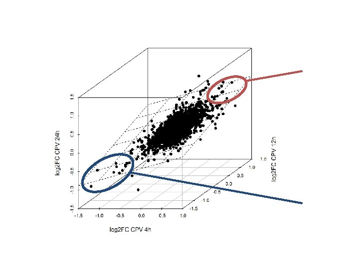
La risposta a CPV è simile fra i tre time points

Ma in realtà – come spesso accade – il grosso del macchinario trascrizionale resta inalterato

La risposta a CPV è simile fra i tre time points

La risposta a CPV è simile fra i tre time points Trascritti indotti da CPV in tutti i time points 9 genes - 3 LEA genes (chaperones and antifreeze, antidrought proteins, , regulated by abscisic acid -ABA- pathway) Hundertmark & Hincha, 2008 Trascritti repressi da CPV 14 genes - 3 peroxidases General stress response peroxidases. The same are repressed by 10 u. M ABA treatment of seedlings (Kim et al. , 2011)

Tempistiche di risposta trascrizionale a CPV Geni alterati (Log 2 FC>0. 5) in almeno uno dei trattamenti CPV

Geni Early Induction Geni Early Repression Transcription factors, laccases, several pectin degradation genes, a LEA protein Chaperonina Hsp 20; invertase/pectin methylesterase inhibitor; metacaspasi 2; Unknown genes Geni a risposta immediata, specifici della fase early

Geni Late Induction Cell wall rearrangement Geni Late Repression ABC transporter; peroxidases Geni specifici della fase late

Scomposizione dell’effetto di CPV Federico Antonietta Risposta a CPV Da ora useremo tutti e tre i time points come replicati vs. Tutti i trattamenti pubblicati e gli effetti noti in Arabidopsis thaliana

Condizioni simili al CPV treatment ARR 22 Participates into a His-Asp phosphorelay pathway. Transgenic lines overexpressing ARR 22 (referred to as ARR 22 -ox) showed the characteristic dwarf phenotypes with poorly developed root systems. The results of Northern blot hybridization with selected sets of hormoneresponsive genes suggested that cytokinin responses are selectively attenuated in ARR 22 -ox, while other hormone responses (auxin, ABA and ethylene) occur normally (Kiba et al. , 2004) CPV Trattamento con CPV molto simile (linee ROSSE) al trattamento con ABA (Goda et al. , At. Gen. Express consortium) , e alla risposta fisiologica della pianta allo stress Osmotico. Effetto opposto (linea BLU) al trattamento con Norflurazon e all’overespressore ARR 22

Condizioni simili al CPV treatment Score Experiment Genotype Treatment / Tissue 0 CPV treatment Col-0 CPV / Whole plants 1 ABA 3 h Col-0 10 µM ABA / seedling 2 ARR 22 -ox (t-zeatin 3 h) ARR 22 -ox 20 µM t-zeatin / seedling 3 ABA 1 h Col-0 10 µM ABA / seedling 4 Norflurazon Col-0 5 Osmotic Stress 24 h (root) Col-0 6 UV Stress 24 h (shoot) Col-0 7 Salt Stress 24 h (root) Col-0 8 Red/FR Light 45 min Col-0 9 Fe starvation 24 h Col-0 10 Mutant cry 1 5 µM Norflurazon / seedling osmotic stress (300 m. M mannitol) / roots UV-B stress (15 min 1. 8 W/m 2 Philips TL 40 W/12; thereafter recovery) / shoots salt stress (150 m. M Na. Cl) / roots Red Light / seedling Fe starvation / whole roots Continuous white light / seedling Spearman Correlation Control Experimental Category Between Experiment significant fold changes Ctrl Perata Group 1. 00 Basic hormone Mock 3 h 0. 77 treatment of seedlings Cytokinin treatment of Col-0 (t-zeatin 3 h) -0. 70 seedlings Basic hormone Mock 1 h 0. 65 treatment of seedlings Col-0 GEO bulk -0. 65 Stress mock 24 h (root) Stress treatments 0. 63 Stress mock 24 h (shoot) Stress treatments -0. 60 Stress mock 24 h (root) Stress treatments 0. 57 Light treatments 0. 56 Control GEO bulk 0. 56 Col-0 GEO bulk 0. 55 At. CAST experiment similarity method (Sasaki et al. , 2011) note: FARO tool gives similar results (we used At. CAST because it contains more experiments)

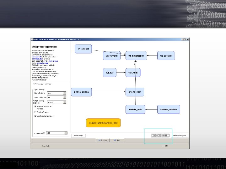
Analisi per pathway CPV 4 ore Risposta simile fra i time points

Analisi per pathway CPV 12 ore Risposta simile fra i time points

Analisi per pathway CPV 24 ore Risposta simile fra i time points

Analisi per pathway Log 2 FC Repressione Perossidasi Induzione via metabolica ABA Degradazione Pectine della Parete Cellulare Glicosil idrolasi Xyloglucano idrolasi Polygalatturonasi

Induzione sintesi antocianine Le antocianine sono da tempo note come metaboliti che si accumulano durante il cold stress, aiutando fra le altre cose nel diminuire la temperature di congelamento (Christie et al. , 1994) Fattori di trascrizione coinvolti (CPV 24 ore) At 1 g 10585 At 2 g 43140 Fattori di trascrizione b. HLH, putativi, risposta robusta nei tre time points Nessun paper specifico li descrive Possibili nuovi candidati genici di risposta trascrizionale

Benché alcune risposte trascrizionali siano condivise, l’effetto di CPV è solo vagamente simile a quello da cold stress (At. Gen. Express consortium) LEA proteins Probabilmente, la risposta a CPV si configura come una mild cold acclimation (ABA-dipendente)

Tutti i dati http: //www. giorgilab. org/biostimolanti/cpv. html Note: the page is not indexed by google, but it is also not encrypted

Conclusioni CPV induce un rilevante incremento delle vie trascrizionali di risposta all’ABA e allo stress osmotico, con livellamento delle piante ad un assetto «late» di preparazione allo stress stesso, probabilmente simile all’acclimazione. L’uso incrociato di 1) Monitoring degli effetti attraverso diversi time points 2) Localizzazione e assegnazione trascritti in pathways 3) Confronto fra i nostri esperimenti e database pubblici ci ha consentito di descrivere l’effetto di CPV nonostante la mancanza di replicati biologici per il trattamento, e la conseguente intrinseca «debolezza» statistica. Questo non solo consente di giustificare almeno in parte gli effetti temperaturaprotettivi di CPV sulle piante, ma indirizza la ricerca verso nuovi potenziali detectors nella risposta vegetale a condizioni di stress, come ad esempio i fattori di trascrizione b. HLH non ancora caratterizzati.

Overview of the course Transcription and Transcriptomics Day 1 23/04/2012 Room β 3

Exercise – set up your R Open the terminal wget http: //www. usadellab. org/cms/uploads/supplementary/trma. tar. gz R CMD INSTALL trma. tar. gz This installs the optional Type R (plus ENTER) You’re now in the R tool for statistics Install the microarray analysis tools: set. Repositories() install. packages("affy. PLM") install. packages("limma") install. packages("plier") And exit: q() Always type y to confirm normalization method This tells R where to find Bioinformatics tools (select «Bio. C software» ) This installs a library for Affymetrix microarray processing This installs a library for differential gene expression analysis