Some considerations on cooling an annular beam distribution

Some considerations on cooling an annular beam distribution Federico Capoani and Massimo Giovannozzi With special thanks to Rogelio Tomás

Introduction Possible applications of manipulating an annular beam distribution: • Re-using spent beam after optics measurements (performed with a transverse kicker). In this case we want to cool the beam emittance, or to push the beam towards the centre of phase space. • Get rid of beam halo by pushing the beam towards the outside of phase space (towards collimators). Stable resonances are certainly an excellent means to perform beam manipulations. So far, resonances have been used to split the beam distribution in a number of parts depending on the order of the stable resonance used (see MTE in the PS). 2/20/2021 M. Giovannozzi | Presentation Title 2

Manipulating an annular beam Two possibilities at hand • Use 1 D resonances generated by magnetic elements • In this way, only the plane in which the beam is annular is affected. • Use 2 D resonances generated by magnetic elements • In this way, both transverse planes are affected. • In fact, the 1 D resonance can be generated by means of an AC dipole, whose frequency is in resonance with the machine tune. This is not considered here… 2/20/2021 M. Giovannozzi | Presentation Title 3

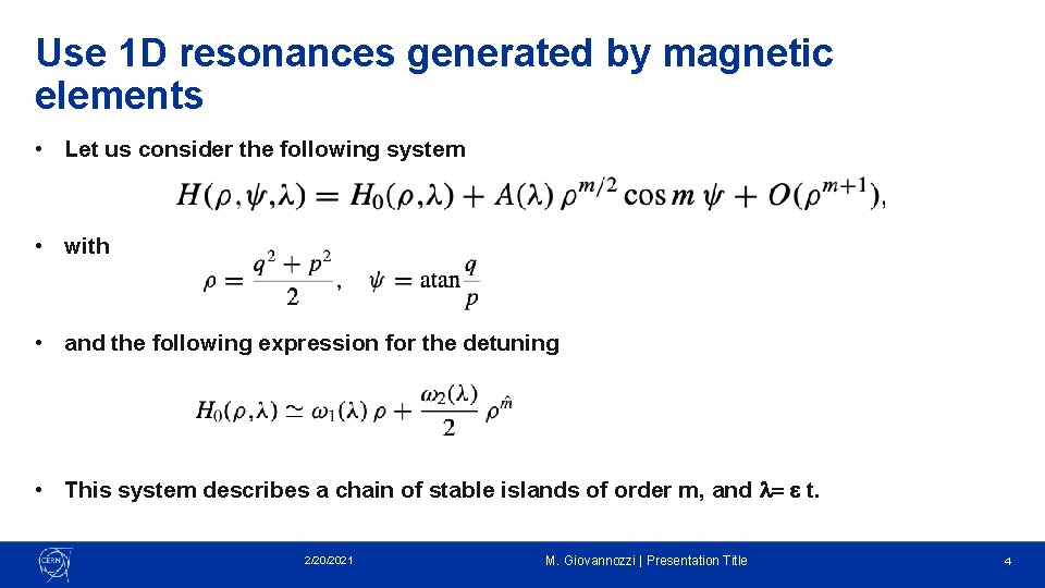
Use 1 D resonances generated by magnetic elements • Let us consider the following system • with • and the following expression for the detuning • This system describes a chain of stable islands of order m, and l= e t. 2/20/2021 M. Giovannozzi | Presentation Title 4

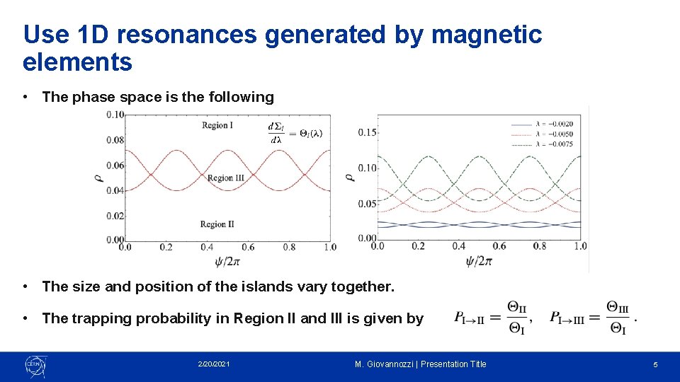
Use 1 D resonances generated by magnetic elements • The phase space is the following • The size and position of the islands vary together. • The trapping probability in Region II and III is given by 2/20/2021 M. Giovannozzi | Presentation Title 5

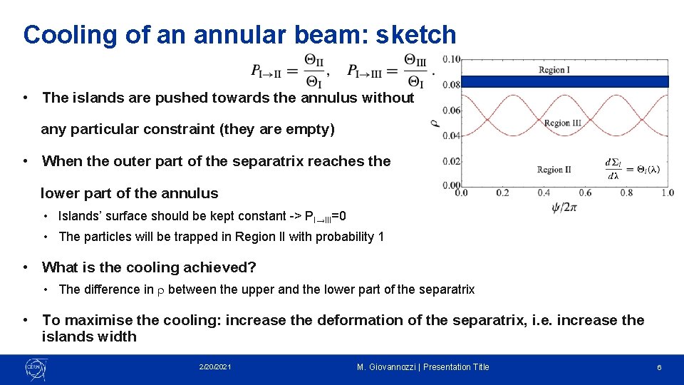
Cooling of an annular beam: sketch • The islands are pushed towards the annulus without any particular constraint (they are empty) • When the outer part of the separatrix reaches the lower part of the annulus • Islands’ surface should be kept constant -> PI→III=0 • The particles will be trapped in Region II with probability 1 • What is the cooling achieved? • The difference in r between the upper and the lower part of the separatrix • To maximise the cooling: increase the deformation of the separatrix, i. e. increase the islands width 2/20/2021 M. Giovannozzi | Presentation Title 6

Cooling of an annular beam: sketch To fix some ideas: • Select the fourth-order resonance: it is stable, but the elliptic and hyperbolic fixed points have different amplitudes. • Use the tune, the sextupole strength, and the octupole strength to control islands’ parameters (statically and dynamically). • Possibly, make the resonance unstable, by cancelling the detuning with amplitude, as this pushes the hyperbolic fixed points very close to the origin, thus increasing the islands width. 2/20/2021 M. Giovannozzi | Presentation Title 7

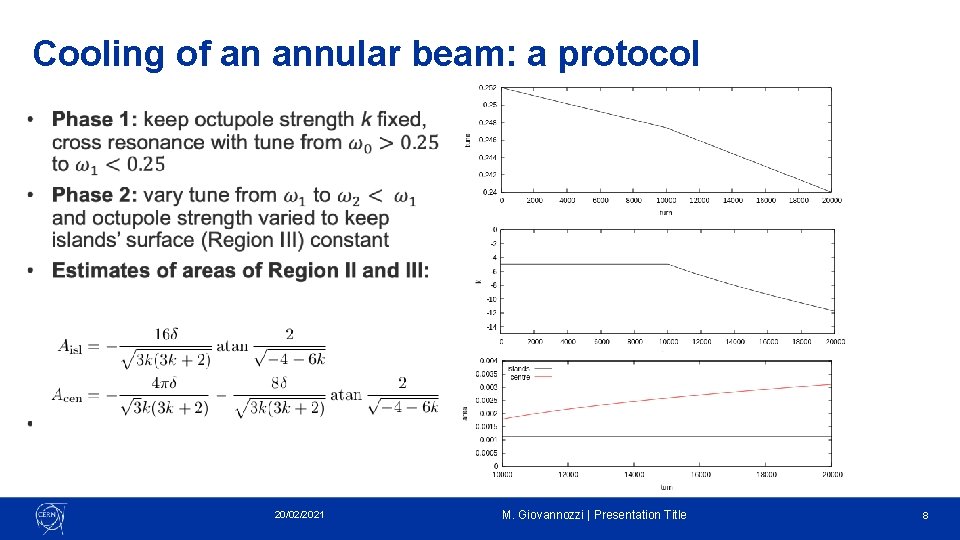
Cooling of an annular beam: a protocol 20/02/2021 M. Giovannozzi | Presentation Title 8

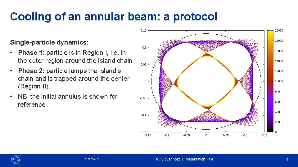
Cooling of an annular beam: a protocol Single-particle dynamics: • Phase 1: particle is in Region I, i. e. in the outer region around the island chain • Phase 2: particle jumps the island’s chain and is trapped around the center (Region II). • NB: the initial annulus is shown for reference 20/02/2021 M. Giovannozzi | Presentation Title 9

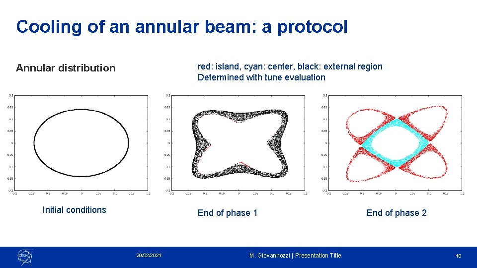
Cooling of an annular beam: a protocol red: island, cyan: center, black: external region Determined with tune evaluation Annular distribution Initial conditions End of phase 1 20/02/2021 M. Giovannozzi | Presentation Title End of phase 2 10

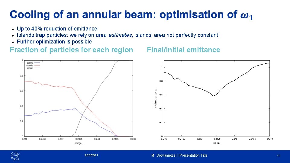
Up to 40% reduction of emittance Islands trap particles: we rely on area estimates, islands’ area not perfectly constant! Further optimization is possible Fraction of particles for each region 2/20/2021 Final/initial emittance M. Giovannozzi | Presentation Title 11

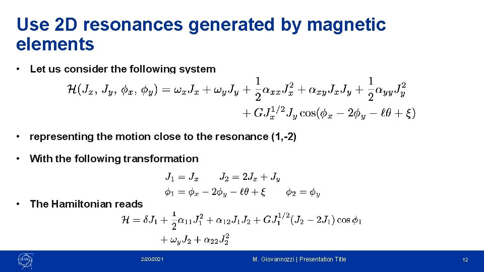
Use 2 D resonances generated by magnetic elements • Let us consider the following system • representing the motion close to the resonance (1, -2) • With the following transformation • The Hamiltonian reads 2/20/2021 M. Giovannozzi | Presentation Title 12

Use 2 D resonances generated by magnetic elements • J 2 is an invariant of motion, which implies that Jx and Jy variations (and emittances) should occur in opposite directions to keep J 2 constant. • This is a generic behaviour for a generic (m, -n) nonlinear resonance. • It can be used for our purpose! 2/20/2021 M. Giovannozzi | Presentation Title 13

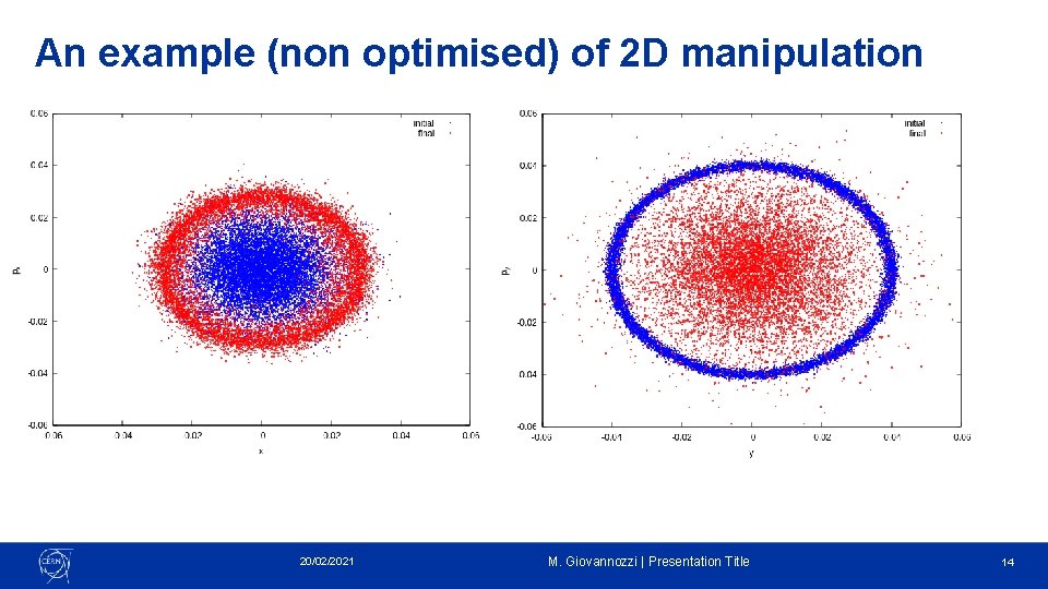
An example (non optimised) of 2 D manipulation 20/02/2021 M. Giovannozzi | Presentation Title 14

Conclusions • Options to cool an annular beam distribution exist: • Use 1 D resonances generated by magnetic elements • Preliminary results are encouraging, using an infinitely thin annular distribution • Optimisation of protocol to be pursued: • adiabaticity of protocol • optimisation of tune values for phase 1 and 2 • Use of exciters (AC dipole or quadrupole) • Not considered, yet, but they will be considered in the future • Use 2 D resonances generated by magnetic elements • It works, but it increases the emittance in the other plane: this is unavoidable, but it might be nevertheless useful 2/20/2021 M. Giovannozzi | Presentation Title 15

home. cern