The Joint Pricing of Volatility and Liquidity Federico

The Joint Pricing of Volatility and Liquidity Federico Bandi, Claudia Moise, Jeffrey Russell Chicago Booth and Case Western Reserve University Summer Meeting of the Econometric Society June 6, 2009

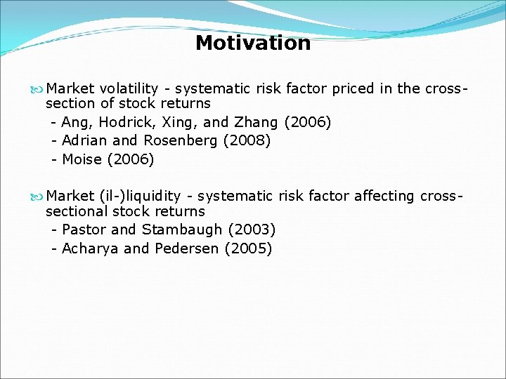
Motivation Market volatility - systematic risk factor priced in the crosssection of stock returns - Ang, Hodrick, Xing, and Zhang (2006) - Adrian and Rosenberg (2008) - Moise (2006) Market (il-)liquidity - systematic risk factor affecting crosssectional stock returns - Pastor and Stambaugh (2003) - Acharya and Pedersen (2005)

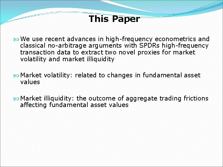
This Paper We use recent advances in high-frequency econometrics and classical no-arbitrage arguments with SPDRs high-frequency transaction data to extract two novel proxies for market volatility and market illiquidity Market volatility: related to changes in fundamental asset values Market illiquidity: the outcome of aggregate trading frictions affecting fundamental asset values

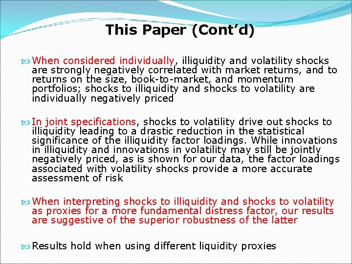
This Paper (Cont’d) When considered individually, illiquidity and volatility shocks are strongly negatively correlated with market returns, and to returns on the size, book-to-market, and momentum portfolios; shocks to illiquidity and shocks to volatility are individually negatively priced In joint specifications, shocks to volatility drive out shocks to illiquidity leading to a drastic reduction in the statistical significance of the illiquidity factor loadings. While innovations in illiquidity and innovations in volatility may still be jointly negatively priced, as is shown for our data, the factor loadings associated with volatility shocks provide a more accurate assessment of risk When interpreting shocks to illiquidity and shocks to volatility as proxies for a more fundamental distress factor, our results are suggestive of the superior robustness of the latter Results hold when using different liquidity proxies

Data: SPDRs High-frequency SPDRs transaction prices (1993 -2005) S&P depository receipts (ownership of a trust which effectively invests in the S&P 500 index) Trade like a stock on the Amex Are exchange traded funds (ETFs) Simple arbitrage considerations imply that they should trade near net asset value (NAV) The deviations from NAV signal market frictions rendering arbitrages harder to implement (Elton, Gruber, Comer, and Li, 2002, Engle and Sarkar, 2002)

Data: SPDRs (Cont’d) Importantly, rather than focusing on deviations of SPDRs trade prices from NAVs, we measure deviations from unobserved fundamental values Using unobserved fundamental values as benchmarks is important (Engle and Sarkar, 2002). The NAV is evaluated at transaction prices. It is well-known from classical market microstructure theory that transaction prices differ from fundamental values. The size of these deviations depends on liquidity Hence, aggregate illiquidity may affect both the size of the deviations between SPDRs prices and NAVs (given the previous arbitrage arguments), and the size of the deviations between the transaction prices of the underlying securities (which lead to the NAVs) and unobserved fundamental values. Lower aggregate liquidity may therefore be expected to lead to larger overall deviations

A Typical Quote “ Some investors appear to believe that the liquidity of an ETF is dependent on the fund's average trading volume, or the number of shares traded per day. However, this is not the case. Rather, a better measure of ETF liquidity is the liquidity of the underlying stocks in the index “ (Yahoo Finance)

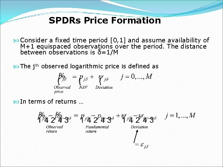
SPDRs Price Formation Consider a fixed time period [0, 1] and assume availability of M+1 equispaced observations over the period. The distance between observations is δ=1/M The jth observed logarithmic price is defined as In terms of returns …

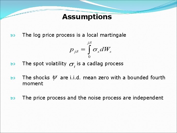
Assumptions The log price process is a local martingale The spot volatility The shocks moment The price process and the noise process are independent is a cadlag process are i. i. d. mean zero with a bounded fourth

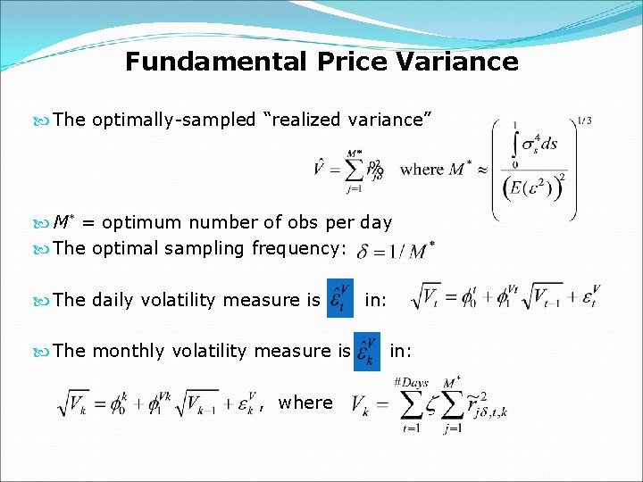
Fundamental Price Variance The optimally-sampled “realized variance” M* = optimum number of obs per day The optimal sampling frequency: The daily volatility measure is The monthly volatility measure is , where in:

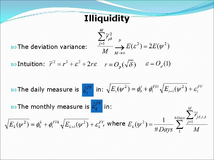
Illiquidity The deviation variance: Intuition: The daily measure is The monthly measure is in: , where

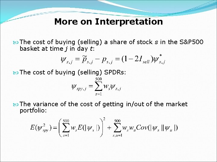
More on Interpretation The cost of buying (selling) a share of stock s in the S&P 500 basket at time j in day t: The cost of buying (selling) SPDRs: The variance of the cost of getting in/out of the market portfolio:

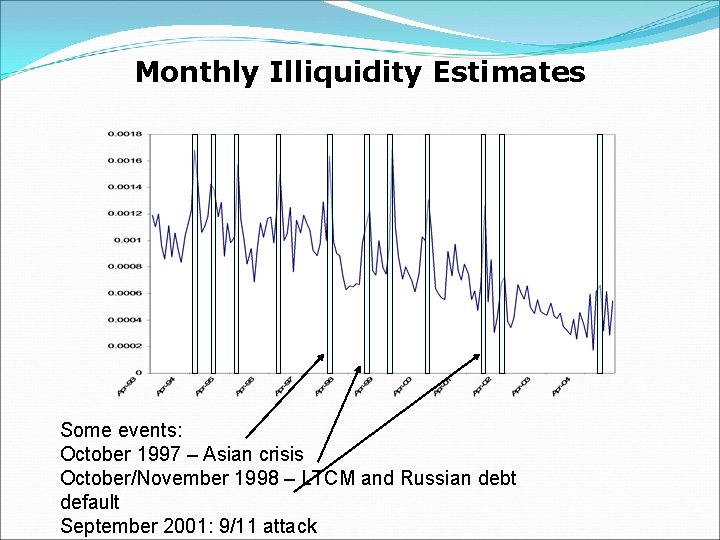
Monthly Illiquidity Estimates Some events: October 1997 – Asian crisis October/November 1998 – LTCM and Russian debt default September 2001: 9/11 attack

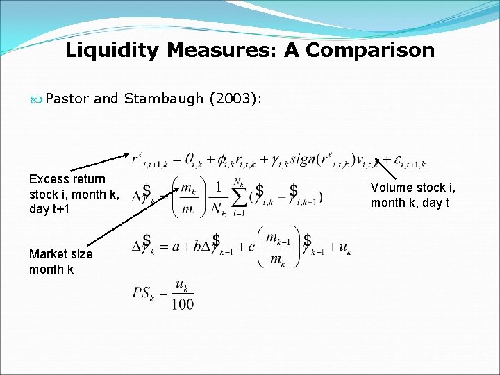
Liquidity Measures: A Comparison Pastor and Stambaugh (2003): Excess return stock i, month k, day t+1 Market size month k Volume stock i, month k, day t

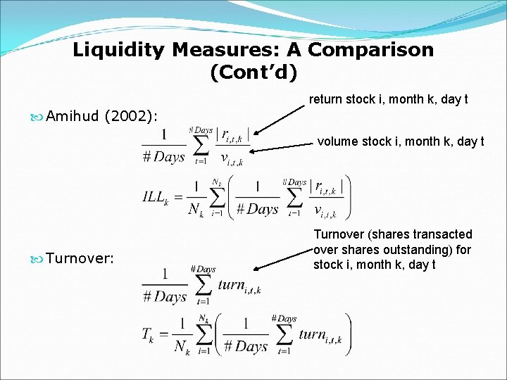
Liquidity Measures: A Comparison (Cont’d) return stock i, month k, day t Amihud (2002): volume stock i, month k, day t Turnover: Turnover (shares transacted over shares outstanding) for stock i, month k, day t

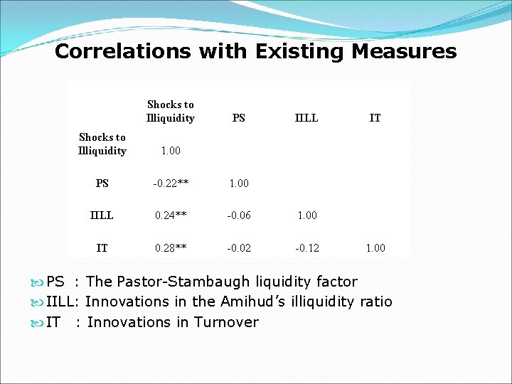
Correlations with Existing Measures Shocks to Illiquidity PS IILL Shocks to Illiquidity 1. 00 PS -0. 22** 1. 00 IILL 0. 24** -0. 06 1. 00 IT 0. 28** -0. 02 -0. 12 IT 1. 00 PS : The Pastor-Stambaugh liquidity factor IILL: Innovations in the Amihud’s illiquidity ratio IT : Innovations in Turnover

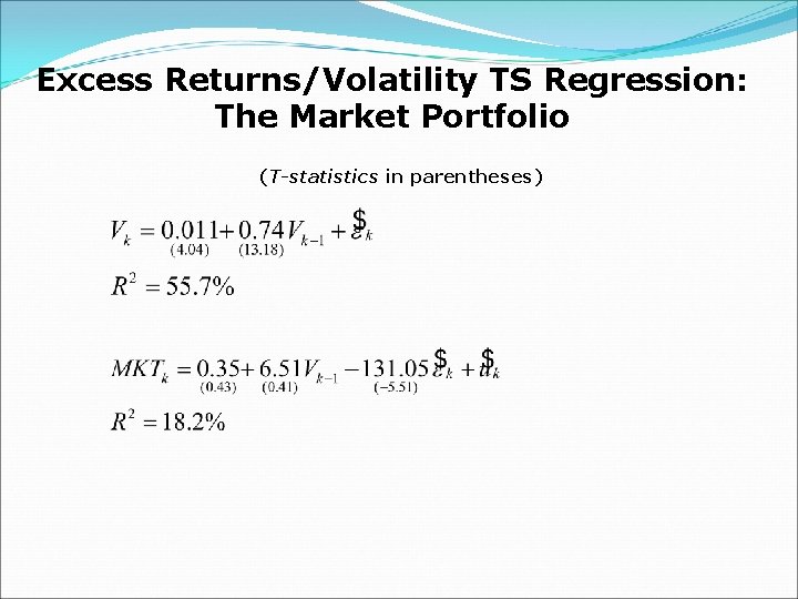
Excess Returns/Volatility TS Regression: The Market Portfolio (T-statistics in parentheses)

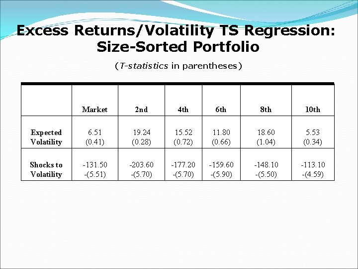
Excess Returns/Volatility TS Regression: Size-Sorted Portfolio (T-statistics in parentheses) Market 2 nd 4 th 6 th 8 th 10 th Expected Volatility 6. 51 (0. 41) 19. 24 (0. 28) 15. 52 (0. 72) 11. 80 (0. 66) 18. 60 (1. 04) 5. 53 (0. 34) Shocks to Volatility -131. 50 -(5. 51) -203. 60 -(5. 70) -177. 20 -(5. 70) -159. 60 -(5. 90) -148. 10 -(5. 50) -113. 10 -(4. 59)

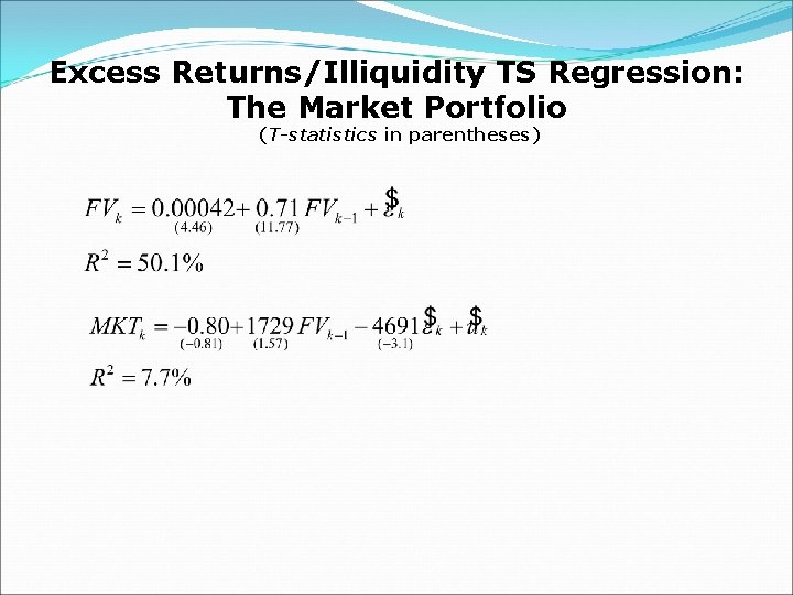
Excess Returns/Illiquidity TS Regression: The Market Portfolio (T-statistics in parentheses)

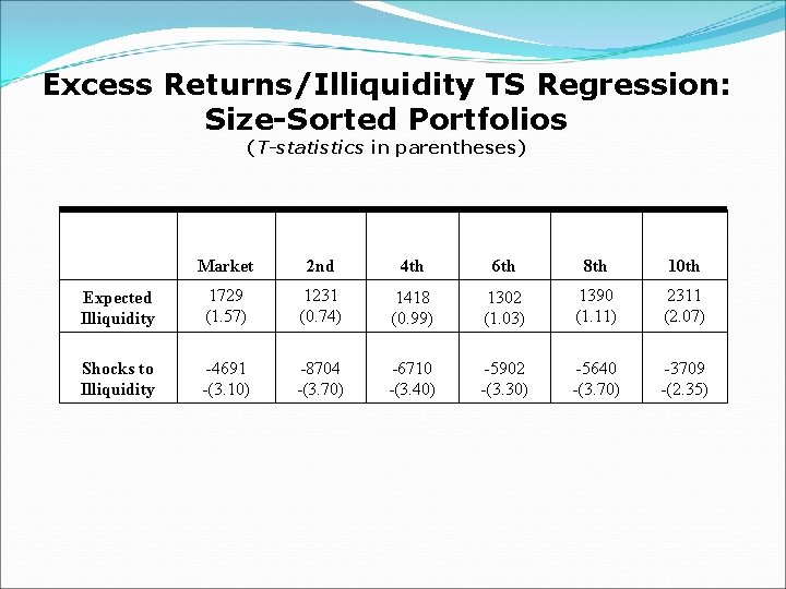
Excess Returns/Illiquidity TS Regression: Size-Sorted Portfolios (T-statistics in parentheses) Market 2 nd 4 th 6 th 8 th 10 th Expected Illiquidity 1729 (1. 57) 1231 (0. 74) 1418 (0. 99) 1302 (1. 03) 1390 (1. 11) 2311 (2. 07) Shocks to Illiquidity -4691 -(3. 10) -8704 -(3. 70) -6710 -(3. 40) -5902 -(3. 30) -5640 -(3. 70) -3709 -(2. 35)

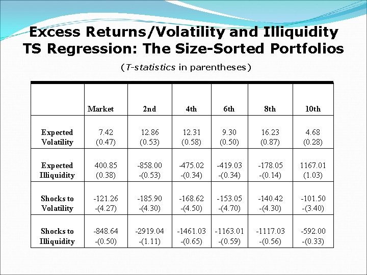
Excess Returns/Volatility and Illiquidity TS Regression: The Size-Sorted Portfolios (T-statistics in parentheses) Market 2 nd 4 th 6 th 8 th 10 th Expected Volatility 7. 42 (0. 47) 12. 86 (0. 53) 12. 31 (0. 58) 9. 30 (0. 50) 16. 23 (0. 87) 4. 68 (0. 28) Expected Illiquidity 400. 85 (0. 38) -858. 00 -(0. 53) -475. 02 -(0. 34) -419. 03 -(0. 34) -178. 05 -(0. 14) 1167. 01 (1. 03) Shocks to Volatility -121. 26 -(4. 27) -185. 90 -(4. 30) -168. 62 -(4. 50) -153. 05 -(4. 70) -140. 42 -(4. 30) -101. 50 -(3. 40) Shocks to Illiquidity -848. 64 -(0. 50) -2919. 04 -(1. 11) -1461. 03 -(0. 65) -1163. 01 -(0. 59) -1117. 03 -(0. 56) -592. 00 -(0. 33)

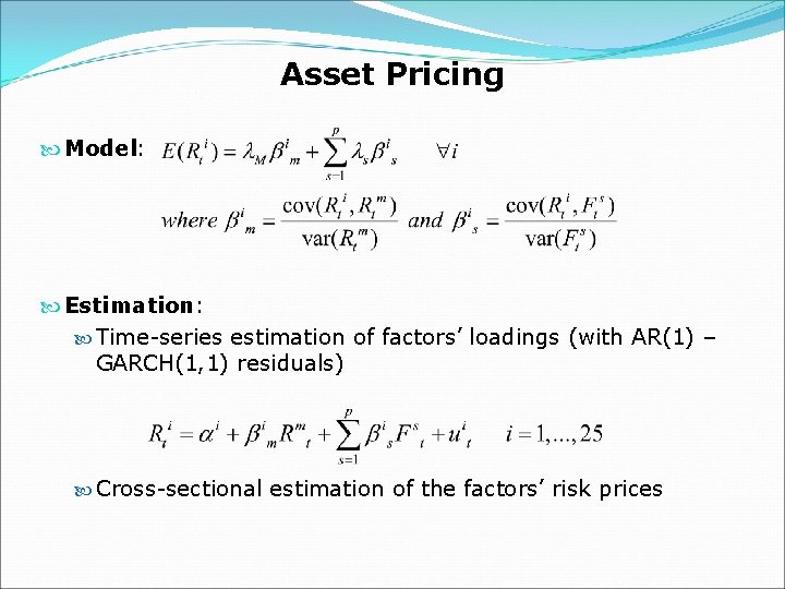
Asset Pricing Model: Estimation: Time-series estimation of factors’ loadings (with AR(1) – GARCH(1, 1) residuals) Cross-sectional estimation of the factors’ risk prices

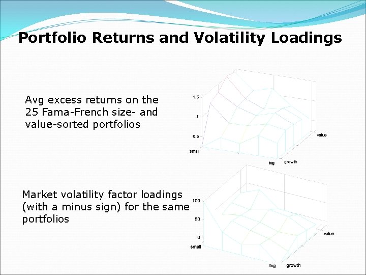
Portfolio Returns and Volatility Loadings Avg excess returns on the 25 Fama-French size- and value-sorted portfolios Market volatility factor loadings (with a minus sign) for the same portfolios

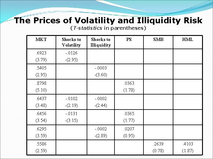
The Prices of Volatility and Illiquidity Risk (T-statistics in parentheses) MKT Shocks to Volatility . 6923 (3. 79) -. 0126 -(2. 95) . 5405 (2. 95) Shocks to Illiquidity HML . 2639 (0. 78) . 4103 (1. 87) . 0363 (1. 78) . 6437 (3. 48) -. 0102 -(2. 19) . 6456 (3. 54) -. 0131 -(3. 15) . 5586 (2. 59) SMB -. 0003 -(3. 60) . 8798 (5. 10) . 6295 (3. 59) PS -. 0002 -(2. 44). 0365 (1. 77) -. 0002 -(2. 89) . 0207 (0. 95)

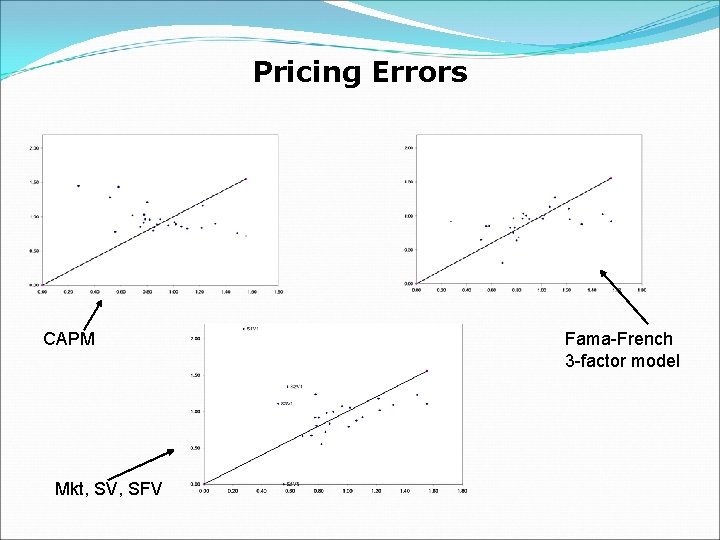
Pricing Errors CAPM Mkt, SV, SFV Fama-French 3 -factor model

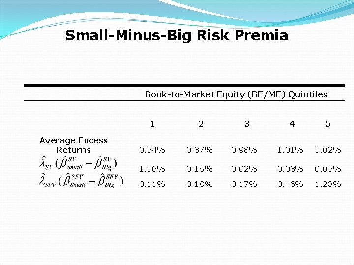
Small-Minus-Big Risk Premia Book-to-Market Equity (BE/ME) Quintiles Average Excess Returns 1 2 0. 54% 0. 87% 1. 16% 0. 11% 3 4 5 0. 98% 1. 01% 1. 02% 0. 16% 0. 02% 0. 08% 0. 05% 0. 18% 0. 17% 0. 46% 1. 28%

Conclusion We extract market-wide volatility and (il-)liquidity proxies from a single time-series of SPDRs high-frequency transaction prices We evaluate the joint cross-sectional pricing implications of volatility and illiquidity using the 25 Fama-French portfolios as test assets Shocks to illiquidity and shocks to volatility are priced in the cross-section of stock returns with a negative sign For our data, we find that the pricing performance of a three factor model with market returns and two volatility components is similar to the pricing performance of the Fama-French 3 -factor model

Conclusion (Cont’d) When jointly considered, shocks to volatility subsume the information contained in shocks to illiquidity (the resulting factor loadings are more accurately estimated) When interpreting illiquidity and volatility as proxies for a more fundamental distress factor, our results are suggestive of the superior robustness of the latter