THE MATHEMATICS OF CAUSAL INFERENCE Judea Pearl Department

THE MATHEMATICS OF CAUSAL INFERENCE Judea Pearl Department of Computer Science UCLA

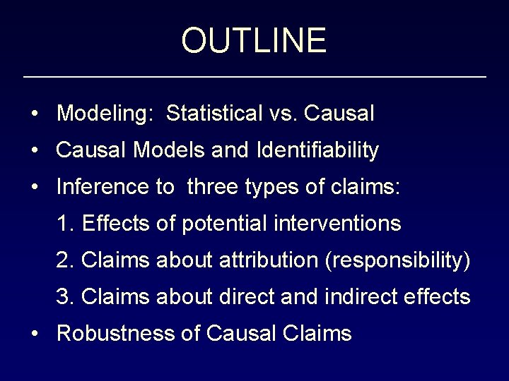
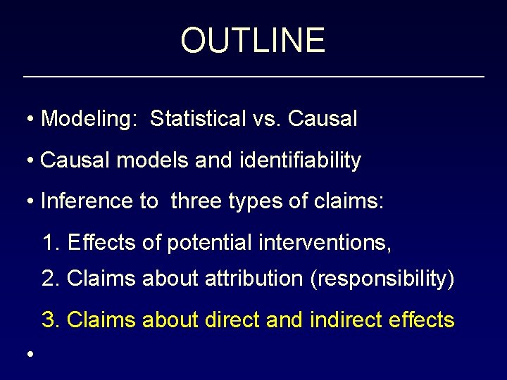
OUTLINE • Modeling: Statistical vs. Causal • Causal Models and Identifiability • Inference to three types of claims: 1. Effects of potential interventions 2. Claims about attribution (responsibility) 3. Claims about direct and indirect effects • Robustness of Causal Claims

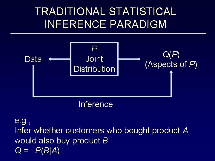
TRADITIONAL STATISTICAL INFERENCE PARADIGM Data P Joint Distribution Q(P) (Aspects of P) Inference e. g. , Infer whether customers who bought product A would also buy product B. Q = P(B|A)

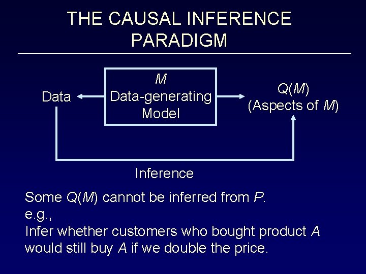
THE CAUSAL INFERENCE PARADIGM Data-generating Model Q(M) (Aspects of M) Inference Some Q(M) cannot be inferred from P. e. g. , Infer whether customers who bought product A would still buy A if we double the price.

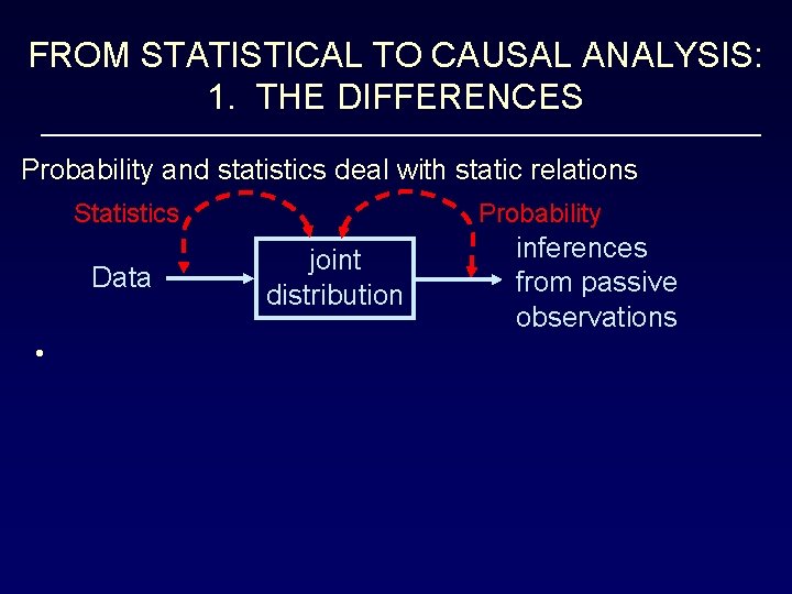
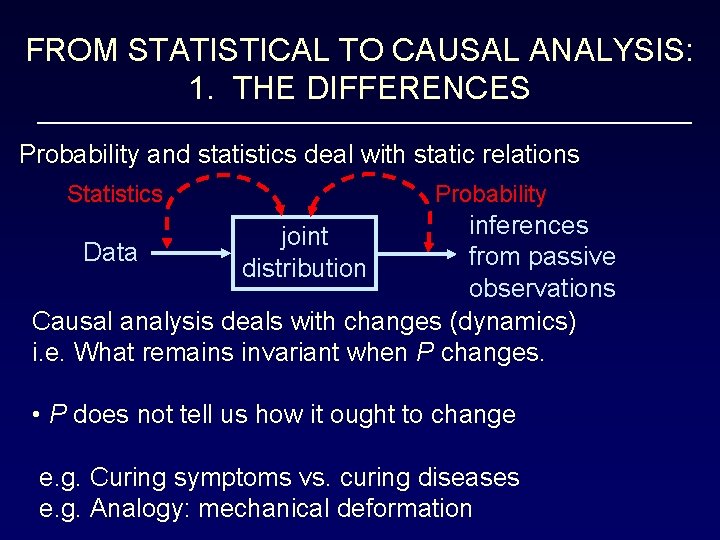
FROM STATISTICAL TO CAUSAL ANALYSIS: 1. THE DIFFERENCES Probability and statistics deal with static relations Statistics Data • Probability joint distribution inferences from passive observations

FROM STATISTICAL TO CAUSAL ANALYSIS: 1. THE DIFFERENCES Probability and statistics deal with static relations Statistics Probability inferences Data from passive observations Causal analysis deals with changes (dynamics) i. e. What remains invariant when P changes. joint distribution • P does not tell us how it ought to change e. g. Curing symptoms vs. curing diseases e. g. Analogy: mechanical deformation

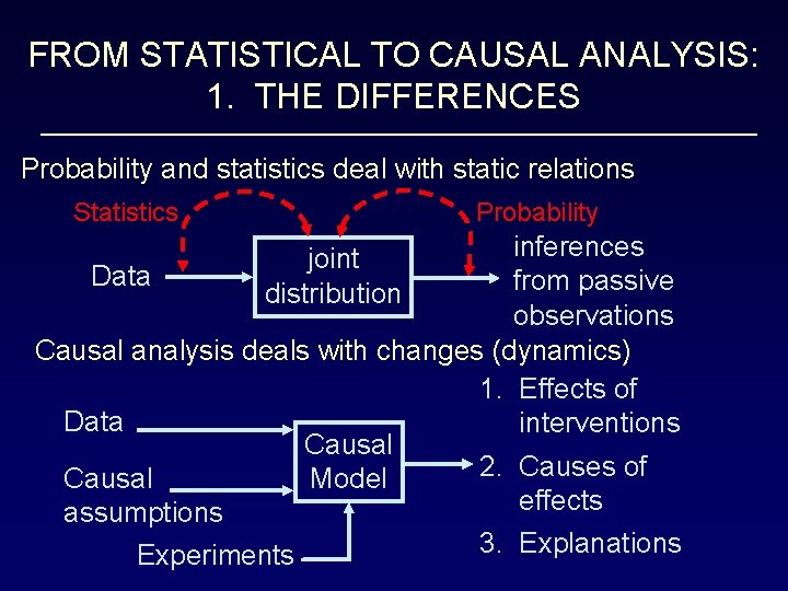
FROM STATISTICAL TO CAUSAL ANALYSIS: 1. THE DIFFERENCES Probability and statistics deal with static relations Statistics Probability inferences Data from passive observations Causal analysis deals with changes (dynamics) 1. Effects of Data interventions Causal 2. Causes of Model Causal effects assumptions 3. Explanations Experiments joint distribution

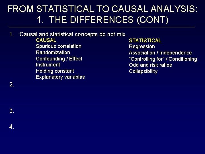
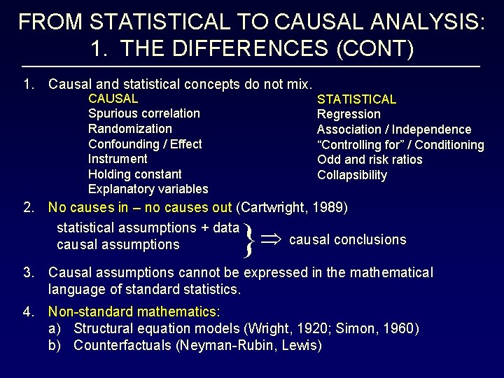
FROM STATISTICAL TO CAUSAL ANALYSIS: 1. THE DIFFERENCES (CONT) 1. Causal and statistical concepts do not mix. CAUSAL Spurious correlation Randomization Confounding / Effect Instrument Holding constant Explanatory variables 2. 3. 4. STATISTICAL Regression Association / Independence “Controlling for” / Conditioning Odd and risk ratios Collapsibility

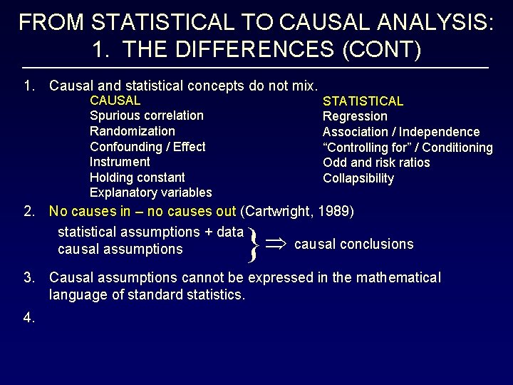
FROM STATISTICAL TO CAUSAL ANALYSIS: 1. THE DIFFERENCES (CONT) 1. Causal and statistical concepts do not mix. CAUSAL Spurious correlation Randomization Confounding / Effect Instrument Holding constant Explanatory variables STATISTICAL Regression Association / Independence “Controlling for” / Conditioning Odd and risk ratios Collapsibility 2. No causes in – no causes out (Cartwright, 1989) statistical assumptions + data causal conclusions causal assumptions } 3. Causal assumptions cannot be expressed in the mathematical language of standard statistics. 4.

FROM STATISTICAL TO CAUSAL ANALYSIS: 1. THE DIFFERENCES (CONT) 1. Causal and statistical concepts do not mix. CAUSAL Spurious correlation Randomization Confounding / Effect Instrument Holding constant Explanatory variables STATISTICAL Regression Association / Independence “Controlling for” / Conditioning Odd and risk ratios Collapsibility 2. No causes in – no causes out (Cartwright, 1989) statistical assumptions + data causal conclusions causal assumptions } 3. Causal assumptions cannot be expressed in the mathematical language of standard statistics. 4. Non-standard mathematics: a) Structural equation models (Wright, 1920; Simon, 1960) b) Counterfactuals (Neyman-Rubin, Lewis)

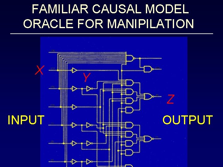
FAMILIAR CAUSAL MODEL ORACLE FOR MANIPILATION X Y Z INPUT OUTPUT

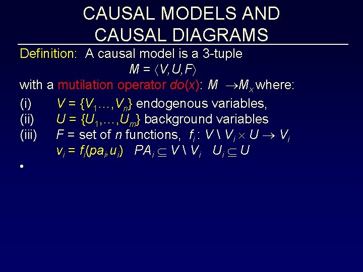
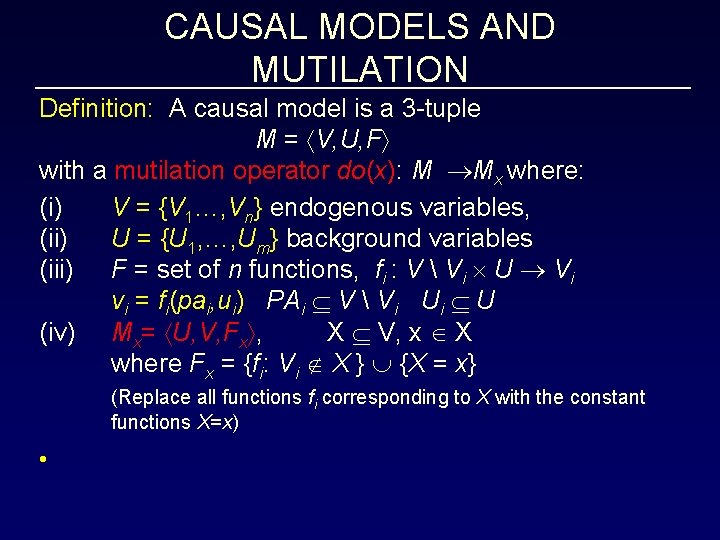
CAUSAL MODELS AND CAUSAL DIAGRAMS Definition: A causal model is a 3 -tuple M = V, U, F with a mutilation operator do(x): M Mx where: (i) V = {V 1…, Vn} endogenous variables, (ii) U = {U 1, …, Um} background variables (iii) F = set of n functions, fi : V Vi U Vi vi = fi(pai, ui) PAi V Vi Ui U •

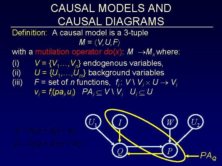
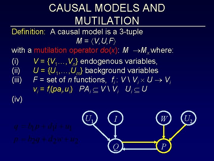
CAUSAL MODELS AND CAUSAL DIAGRAMS Definition: A causal model is a 3 -tuple M = V, U, F with a mutilation operator do(x): M Mx where: (i) V = {V 1…, Vn} endogenous variables, (ii) U = {U 1, …, Um} background variables (iii) F = set of n functions, fi : V Vi U Vi vi = fi(pai, ui) PAi V Vi Ui U U 1 I W Q P U 2 PAQ

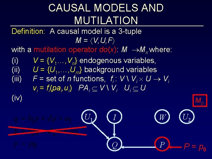
CAUSAL MODELS AND MUTILATION Definition: A causal model is a 3 -tuple M = V, U, F with a mutilation operator do(x): M Mx where: (i) V = {V 1…, Vn} endogenous variables, (ii) U = {U 1, …, Um} background variables (iii) F = set of n functions, fi : V Vi U Vi vi = fi(pai, ui) PAi V Vi Ui U (iv) Mx= U, V, Fx , X V, x X where Fx = {fi: Vi X } {X = x} (Replace all functions fi corresponding to X with the constant functions X=x) •

CAUSAL MODELS AND MUTILATION Definition: A causal model is a 3 -tuple M = V, U, F with a mutilation operator do(x): M Mx where: (i) V = {V 1…, Vn} endogenous variables, (ii) U = {U 1, …, Um} background variables (iii) F = set of n functions, fi : V Vi U Vi vi = fi(pai, ui) PAi V Vi Ui U (iv) U 1 I W Q P U 2

CAUSAL MODELS AND MUTILATION Definition: A causal model is a 3 -tuple M = V, U, F with a mutilation operator do(x): M Mx where: (i) V = {V 1…, Vn} endogenous variables, (ii) U = {U 1, …, Um} background variables (iii) F = set of n functions, fi : V Vi U Vi vi = fi(pai, ui) PAi V Vi Ui U (iv) U 1 Mp I W U 2 Q P P = p 0

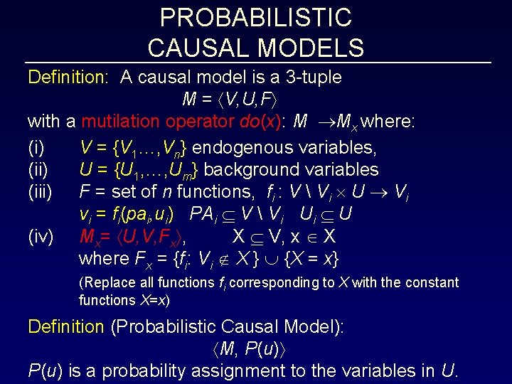
PROBABILISTIC CAUSAL MODELS Definition: A causal model is a 3 -tuple M = V, U, F with a mutilation operator do(x): M Mx where: (i) V = {V 1…, Vn} endogenous variables, (ii) U = {U 1, …, Um} background variables (iii) F = set of n functions, fi : V Vi U Vi vi = fi(pai, ui) PAi V Vi Ui U (iv) Mx= U, V, Fx , X V, x X where Fx = {fi: Vi X } {X = x} (Replace all functions fi corresponding to X with the constant functions X=x) Definition (Probabilistic Causal Model): M, P(u) is a probability assignment to the variables in U.

CAUSAL MODELS AND COUNTERFACTUALS Definition: Potential Response The sentence: “Y would be y (in unit u), had X been x, ” denoted Yx(u) = y, is the solution for Y in a mutilated model Mx, with the equations for X replaced by X = x. (“unit-based potential outcome”) • •

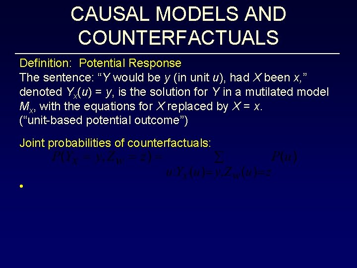
CAUSAL MODELS AND COUNTERFACTUALS Definition: Potential Response The sentence: “Y would be y (in unit u), had X been x, ” denoted Yx(u) = y, is the solution for Y in a mutilated model Mx, with the equations for X replaced by X = x. (“unit-based potential outcome”) Joint probabilities of counterfactuals: •

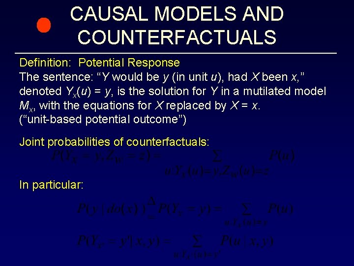
CAUSAL MODELS AND COUNTERFACTUALS Definition: Potential Response The sentence: “Y would be y (in unit u), had X been x, ” denoted Yx(u) = y, is the solution for Y in a mutilated model Mx, with the equations for X replaced by X = x. (“unit-based potential outcome”) Joint probabilities of counterfactuals: In particular:

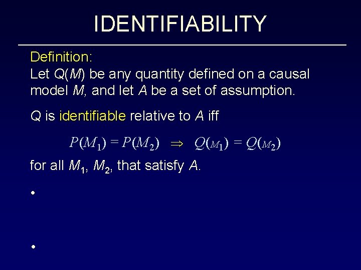
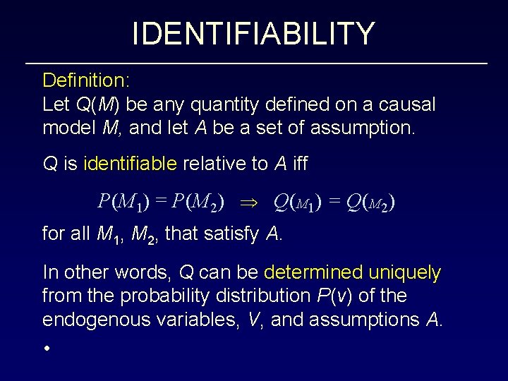
IDENTIFIABILITY Definition: Let Q(M) be any quantity defined on a causal model M, and let A be a set of assumption. Q is identifiable relative to A iff P(M 1) = P(M 2) Q(M 1) = Q(M 2) for all M 1, M 2, that satisfy A. • •

IDENTIFIABILITY Definition: Let Q(M) be any quantity defined on a causal model M, and let A be a set of assumption. Q is identifiable relative to A iff P(M 1) = P(M 2) Q(M 1) = Q(M 2) for all M 1, M 2, that satisfy A. In other words, Q can be determined uniquely from the probability distribution P(v) of the endogenous variables, V, and assumptions A. •

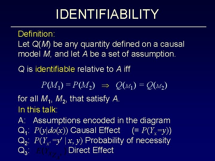
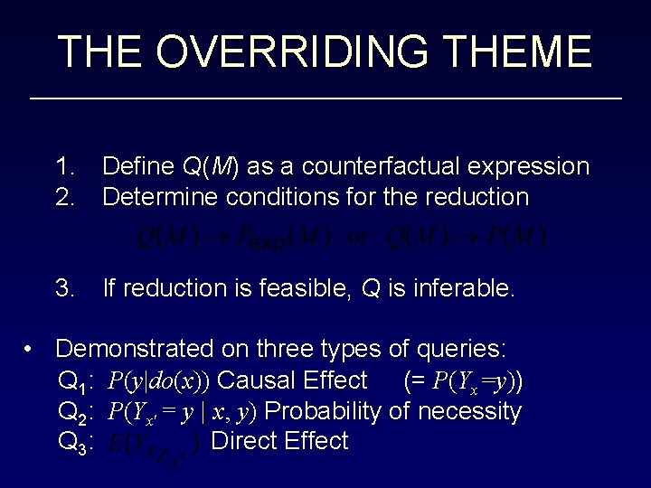
IDENTIFIABILITY Definition: Let Q(M) be any quantity defined on a causal model M, and let A be a set of assumption. Q is identifiable relative to A iff P(M 1) = P(M 2) Q(M 1) = Q(M 2) for all M 1, M 2, that satisfy A. In this talk: A: Assumptions encoded in the diagram Q 1: P(y|do(x)) Causal Effect (= P(Yx=y)) Q 2: P(Yx =y | x, y) Probability of necessity Q 3: Direct Effect

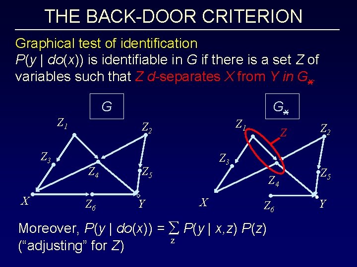
THE BACK-DOOR CRITERION Graphical test of identification P(y | do(x)) is identifiable in G if there is a set Z of variables such that Z d-separates X from Y in Gx. G Z 1 Z 3 X Gx Z 1 Z 2 Z 4 Z 6 Z 3 Z 5 Y Z Z 4 X Z 6 Moreover, P(y | do(x)) = å P(y | x, z) P(z) z (“adjusting” for Z) Z 2 Z 5 Y

OUTLINE • Modeling: Statistical vs. Causal • Causal models and identifiability • Inference to three types of claims: 1. Effects of potential interventions, 2. Claims about attribution (responsibility) 3.

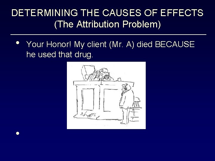
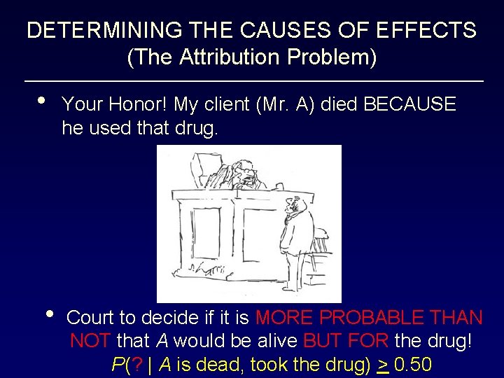
DETERMINING THE CAUSES OF EFFECTS (The Attribution Problem) • • Your Honor! My client (Mr. A) died BECAUSE he used that drug.

DETERMINING THE CAUSES OF EFFECTS (The Attribution Problem) • • Your Honor! My client (Mr. A) died BECAUSE he used that drug. Court to decide if it is MORE PROBABLE THAN NOT that A would be alive BUT FOR the drug! P(? | A is dead, took the drug) > 0. 50

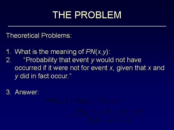
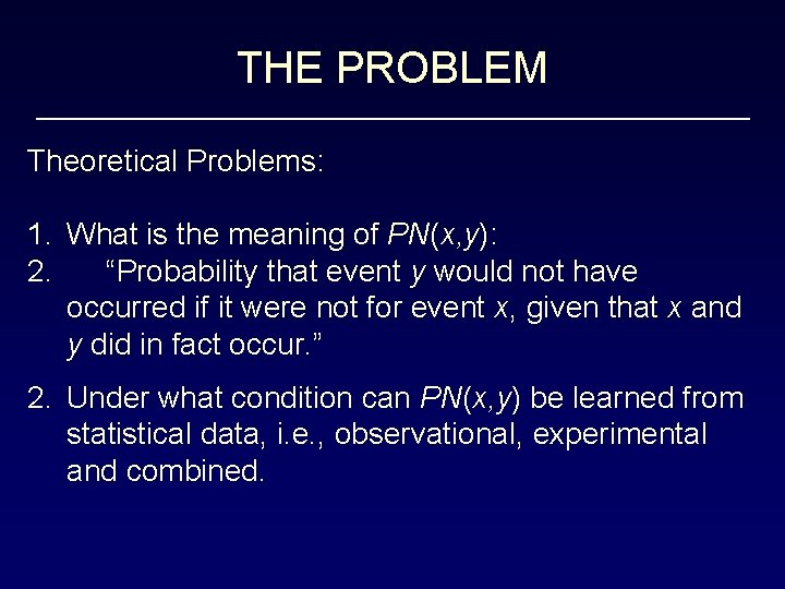
THE PROBLEM Theoretical Problems: 1. What is the meaning of PN(x, y): 2. “Probability that event y would not have occurred if it were not for event x, given that x and y did in fact occur. ” •

THE PROBLEM Theoretical Problems: 1. What is the meaning of PN(x, y): 2. “Probability that event y would not have occurred if it were not for event x, given that x and y did in fact occur. ” 3. Answer:

THE PROBLEM Theoretical Problems: 1. What is the meaning of PN(x, y): 2. “Probability that event y would not have occurred if it were not for event x, given that x and y did in fact occur. ” 2. Under what condition can PN(x, y) be learned from statistical data, i. e. , observational, experimental and combined.

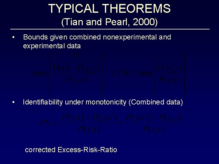
TYPICAL THEOREMS (Tian and Pearl, 2000) • Bounds given combined nonexperimental and experimental data • Identifiability under monotonicity (Combined data) corrected Excess-Risk-Ratio

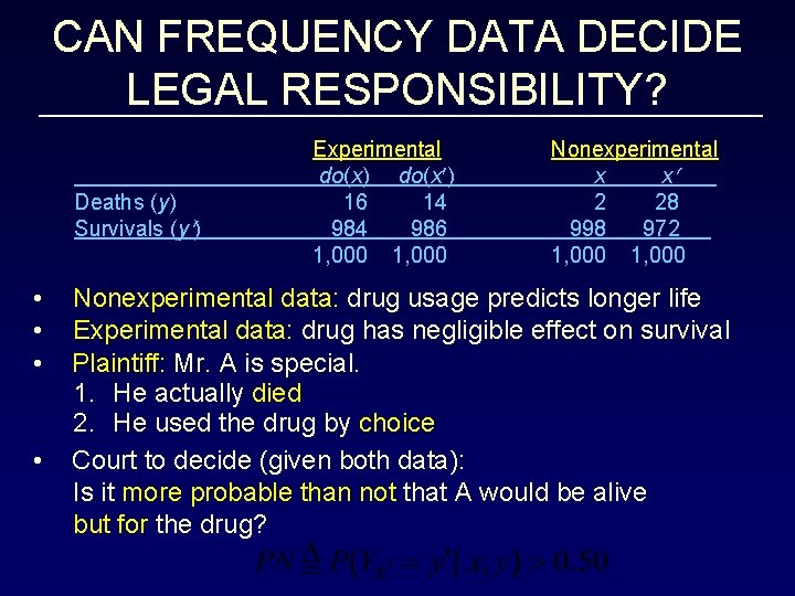
CAN FREQUENCY DATA DECIDE LEGAL RESPONSIBILITY? Deaths (y) Survivals (y ) • • Experimental do(x) do(x ) 16 14 986 1, 000 Nonexperimental x x 2 28 998 972 1, 000 Nonexperimental data: drug usage predicts longer life Experimental data: drug has negligible effect on survival Plaintiff: Mr. A is special. 1. He actually died 2. He used the drug by choice Court to decide (given both data): Is it more probable than not that A would be alive but for the drug?

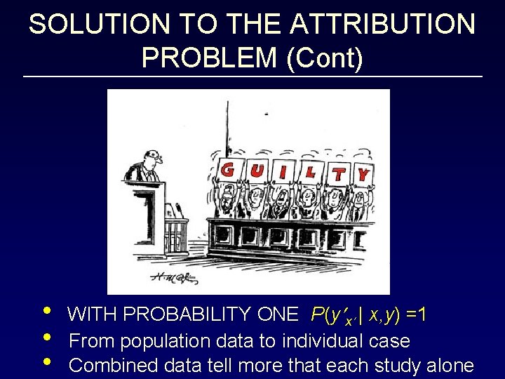
SOLUTION TO THE ATTRIBUTION PROBLEM (Cont) • • • WITH PROBABILITY ONE P(y x | x, y) =1 From population data to individual case Combined data tell more that each study alone

OUTLINE • Modeling: Statistical vs. Causal • Causal models and identifiability • Inference to three types of claims: 1. Effects of potential interventions, 2. Claims about attribution (responsibility) 3. Claims about direct and indirect effects •

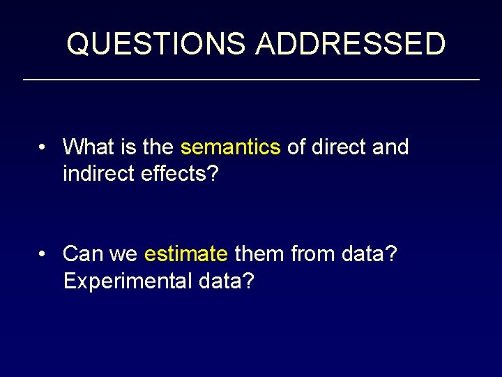
QUESTIONS ADDRESSED • What is the semantics of direct and indirect effects? • Can we estimate them from data? Experimental data?

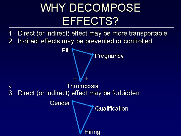
WHY DECOMPOSE EFFECTS? 1. Direct (or indirect) effect may be more transportable. 2. Indirect effects may be prevented or controlled. Pill Pregnancy 3. + + Thrombosis 3. Direct (or indirect) effect may be forbidden Gender Qualification Hiring

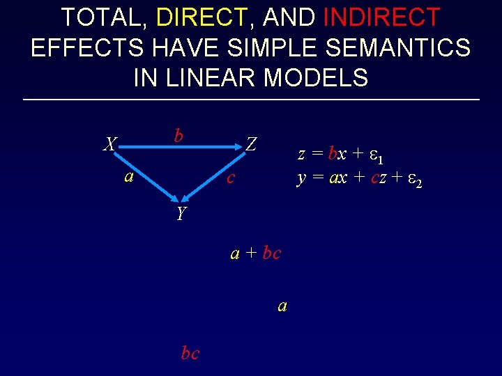
TOTAL, DIRECT, AND INDIRECT EFFECTS HAVE SIMPLE SEMANTICS IN LINEAR MODELS b X a Z z = bx + 1 y = ax + cz + 2 c Y a + bc a bc

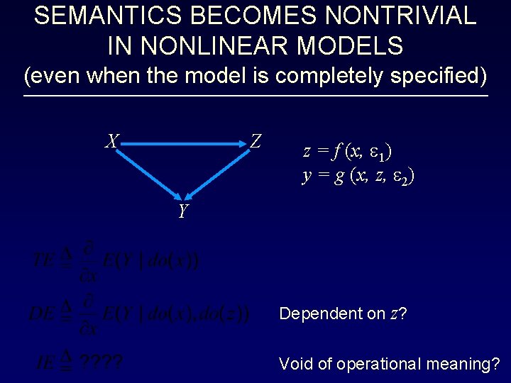
SEMANTICS BECOMES NONTRIVIAL IN NONLINEAR MODELS (even when the model is completely specified) X Z z = f (x, 1) y = g (x, z, 2) Y Dependent on z? Void of operational meaning?

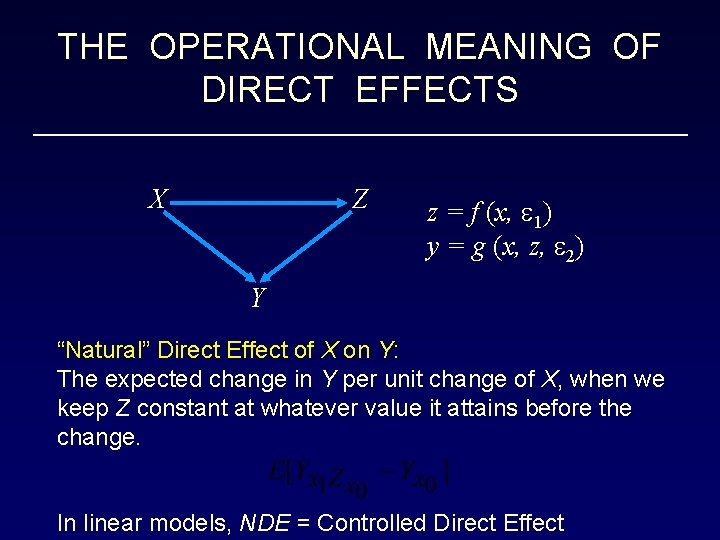
THE OPERATIONAL MEANING OF DIRECT EFFECTS X Z z = f (x, 1) y = g (x, z, 2) Y “Natural” Direct Effect of X on Y: The expected change in Y per unit change of X, when we keep Z constant at whatever value it attains before the change. In linear models, NDE = Controlled Direct Effect

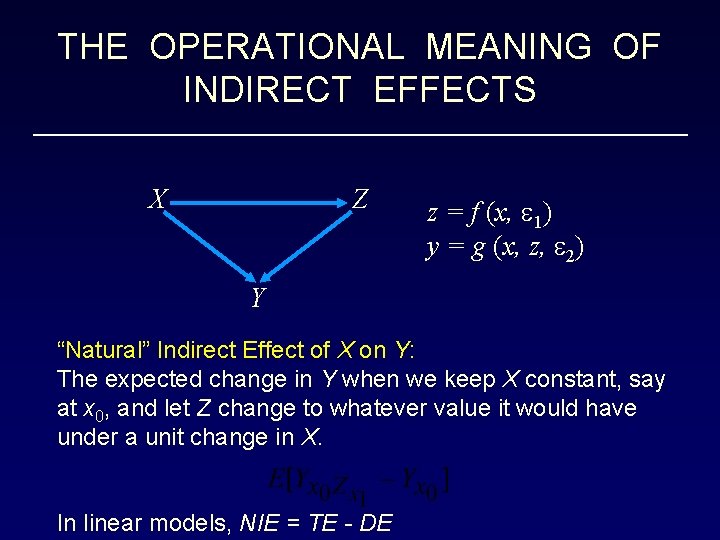
THE OPERATIONAL MEANING OF INDIRECT EFFECTS X Z z = f (x, 1) y = g (x, z, 2) Y “Natural” Indirect Effect of X on Y: The expected change in Y when we keep X constant, say at x 0, and let Z change to whatever value it would have under a unit change in X. In linear models, NIE = TE - DE

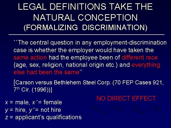
LEGAL DEFINITIONS TAKE THE NATURAL CONCEPTION (FORMALIZING DISCRIMINATION) ``The central question in any employment-discrimination case is whether the employer would have taken the same action had the employee been of different race (age, sex, religion, national origin etc. ) and everything else had been the same’’ [Carson versus Bethlehem Steel Corp. (70 FEP Cases 921, 7 th Cir. (1996))] x = male, x = female y = hire, y = not hire z = applicant’s qualifications NO DIRECT EFFECT

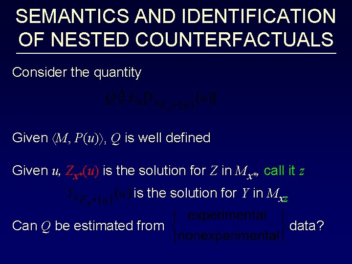
SEMANTICS AND IDENTIFICATION OF NESTED COUNTERFACTUALS Consider the quantity Given M, P(u) , Q is well defined Given u, Zx*(u) is the solution for Z in Mx*, call it z is the solution for Y in Mxz Can Q be estimated from data?

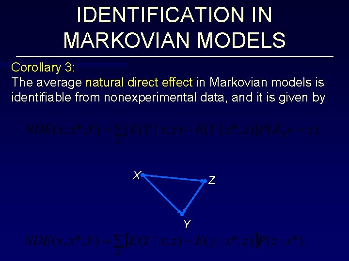
IDENTIFICATION IN MARKOVIAN MODELS Corollary 3: The average natural direct effect in Markovian models is identifiable from nonexperimental data, and it is given by X Z Y

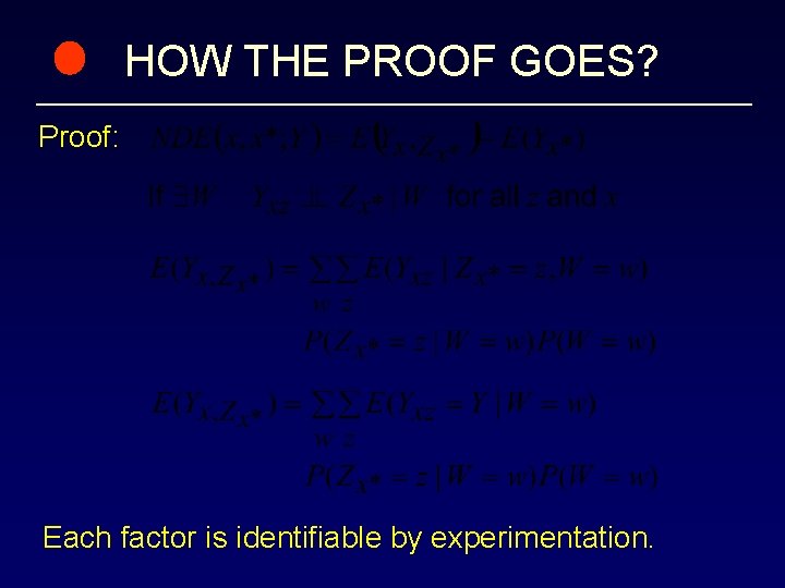
HOW THE PROOF GOES? Proof: Each factor is identifiable by experimentation.

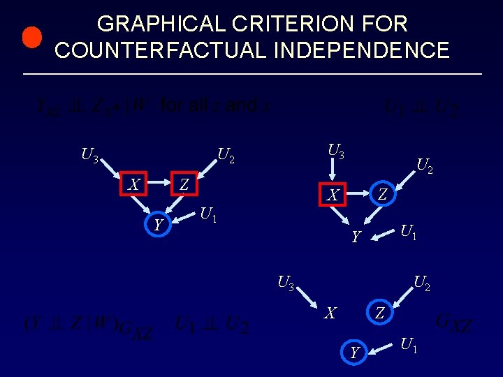
GRAPHICAL CRITERION FOR COUNTERFACTUAL INDEPENDENCE U 3 U 2 X Z Y U 2 Z X U 1 Y U 3 U 2 Z X Y U 1

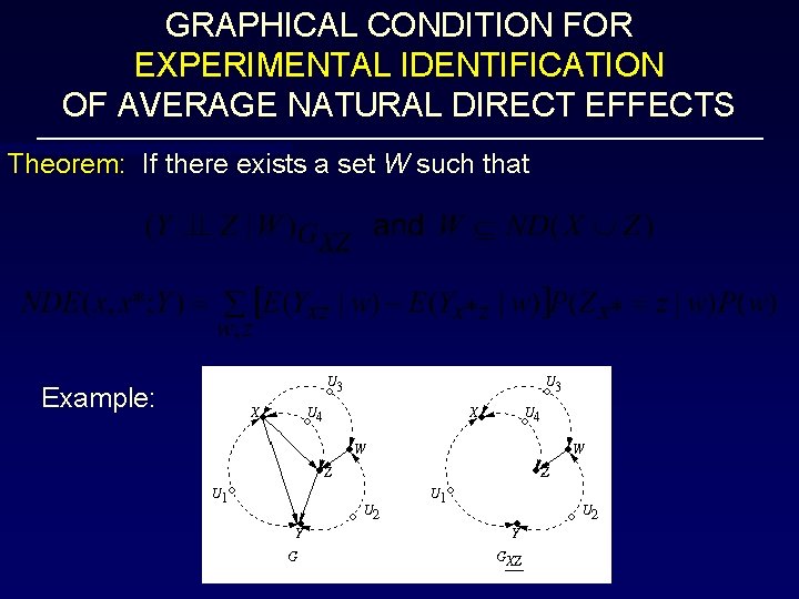
GRAPHICAL CONDITION FOR EXPERIMENTAL IDENTIFICATION OF AVERAGE NATURAL DIRECT EFFECTS Theorem: If there exists a set W such that Example:

THE OVERRIDING THEME 1. Define Q(M) as a counterfactual expression 2. Determine conditions for the reduction 3. If reduction is feasible, Q is inferable. • Demonstrated on three types of queries: Q 1: P(y|do(x)) Causal Effect (= P(Yx=y)) Q 2: P(Yx = y | x, y) Probability of necessity Q 3: Direct Effect

CONCLUSIONS Structural-model semantics enriched with logic + graphs leads to formal interpretation and practical assessments of wide variety of causal and counterfactual relationships.