CAUSAL INFERENCE MATHEMATICAL FOUNDATIONS AND PRACTICAL APPLICATIONS Judea

CAUSAL INFERENCE: MATHEMATICAL FOUNDATIONS AND PRACTICAL APPLICATIONS Judea Pearl University of California Los Angeles (www. cs. ucla. edu/~judea/) 1

OUTLINE • Inference: Statistical vs. Causal, distinctions, and mental barriers • Unified conceptualization of counterfactuals, structural-equations, and graphs • Inference to three types of claims: 1. Effect of potential interventions 2. Attribution (Causes of Effects) 3. Direct and indirect effects (Mediation) • Frills: Transportability, validity, surrogate, etc. 2

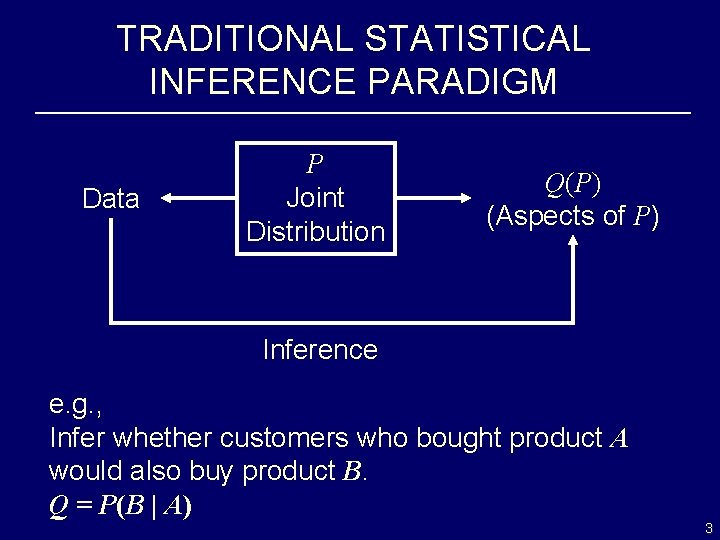
TRADITIONAL STATISTICAL INFERENCE PARADIGM Data P Joint Distribution Q(P) (Aspects of P) Inference e. g. , Infer whether customers who bought product A would also buy product B. Q = P(B | A) 3

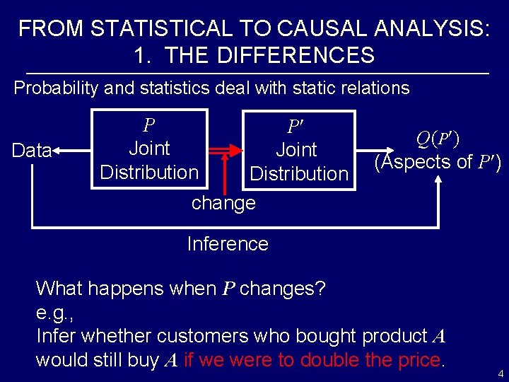
FROM STATISTICAL TO CAUSAL ANALYSIS: 1. THE DIFFERENCES Probability and statistics deal with static relations Data P Joint Distribution change Q(P ) (Aspects of P ) Inference What happens when P changes? e. g. , Infer whether customers who bought product A would still buy A if we were to double the price. 4

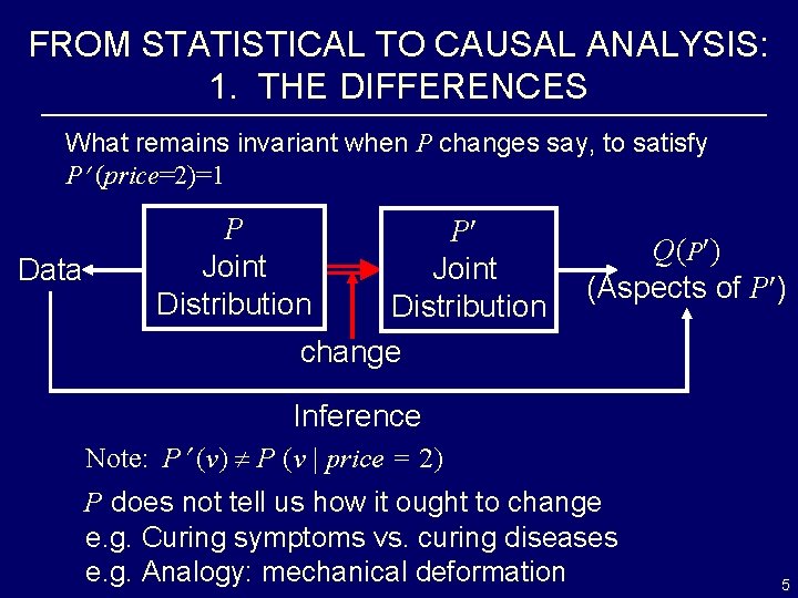
FROM STATISTICAL TO CAUSAL ANALYSIS: 1. THE DIFFERENCES What remains invariant when P changes say, to satisfy P (price=2)=1 Data P Joint Distribution change Q(P ) (Aspects of P ) Inference Note: P (v) P (v | price = 2) P does not tell us how it ought to change e. g. Curing symptoms vs. curing diseases e. g. Analogy: mechanical deformation 5

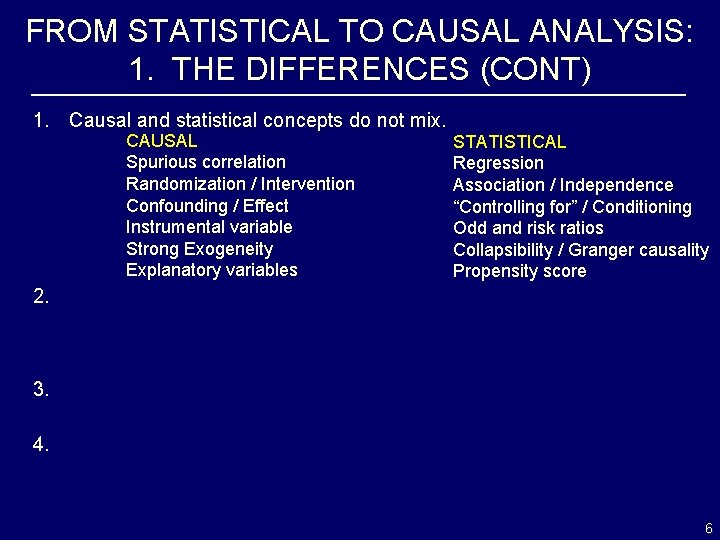
FROM STATISTICAL TO CAUSAL ANALYSIS: 1. THE DIFFERENCES (CONT) 1. Causal and statistical concepts do not mix. CAUSAL Spurious correlation Randomization / Intervention Confounding / Effect Instrumental variable Strong Exogeneity Explanatory variables STATISTICAL Regression Association / Independence “Controlling for” / Conditioning Odd and risk ratios Collapsibility / Granger causality Propensity score 2. 3. 4. 6

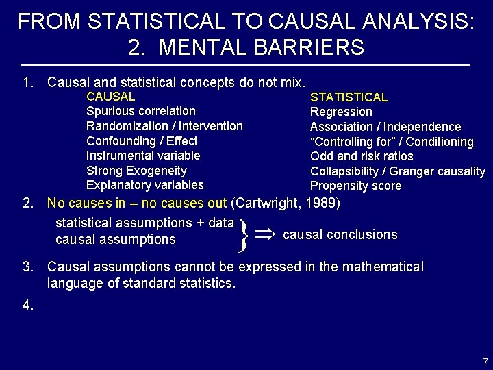
FROM STATISTICAL TO CAUSAL ANALYSIS: 2. MENTAL BARRIERS 1. Causal and statistical concepts do not mix. CAUSAL Spurious correlation Randomization / Intervention Confounding / Effect Instrumental variable Strong Exogeneity Explanatory variables STATISTICAL Regression Association / Independence “Controlling for” / Conditioning Odd and risk ratios Collapsibility / Granger causality Propensity score 2. No causes in – no causes out (Cartwright, 1989) statistical assumptions + data causal conclusions causal assumptions } 3. Causal assumptions cannot be expressed in the mathematical language of standard statistics. 4. 7

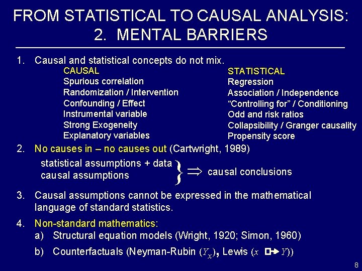
FROM STATISTICAL TO CAUSAL ANALYSIS: 2. MENTAL BARRIERS 1. Causal and statistical concepts do not mix. CAUSAL Spurious correlation Randomization / Intervention Confounding / Effect Instrumental variable Strong Exogeneity Explanatory variables STATISTICAL Regression Association / Independence “Controlling for” / Conditioning Odd and risk ratios Collapsibility / Granger causality Propensity score 2. No causes in – no causes out (Cartwright, 1989) statistical assumptions + data causal conclusions causal assumptions } 3. Causal assumptions cannot be expressed in the mathematical language of standard statistics. 4. Non-standard mathematics: a) Structural equation models (Wright, 1920; Simon, 1960) b) Counterfactuals (Neyman-Rubin (Yx), Lewis (x Y)) 8

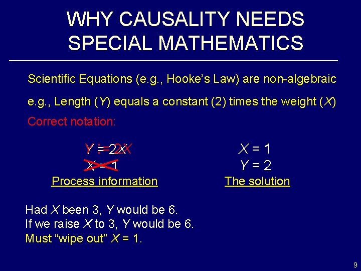
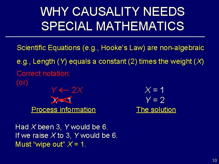
WHY CAUSALITY NEEDS SPECIAL MATHEMATICS Scientific Equations (e. g. , Hooke’s Law) are non-algebraic e. g. , Length (Y) equals a constant (2) times the weight (X) Correct notation: Y : ==2 X 2 X X=1 Y=2 Process information The solution Had X been 3, Y would be 6. If we raise X to 3, Y would be 6. Must “wipe out” X = 1. 9

WHY CAUSALITY NEEDS SPECIAL MATHEMATICS Scientific Equations (e. g. , Hooke’s Law) are non-algebraic e. g. , Length (Y) equals a constant (2) times the weight (X) Correct notation: (or) Y 2 X X=1 Process information X=1 Y=2 The solution Had X been 3, Y would be 6. If we raise X to 3, Y would be 6. Must “wipe out” X = 1. 10

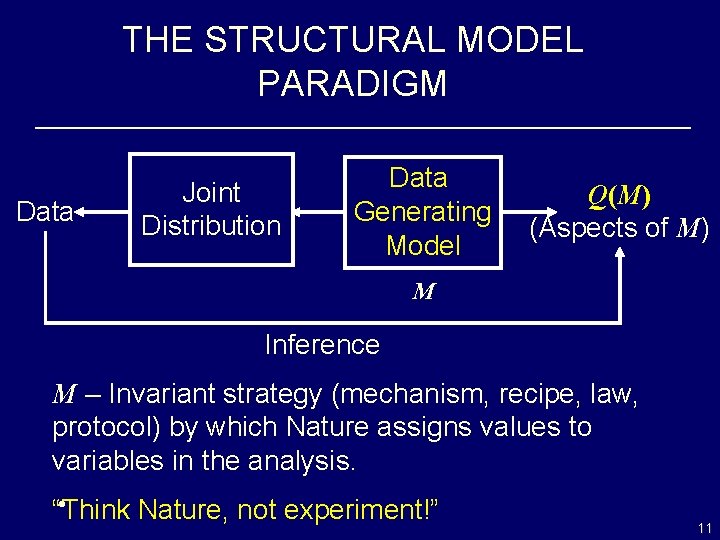
THE STRUCTURAL MODEL PARADIGM Data Joint Distribution Data Generating Model Q(M) (Aspects of M) M Inference M – Invariant strategy (mechanism, recipe, law, protocol) by which Nature assigns values to variables in the analysis. • “Think Nature, not experiment!” 11

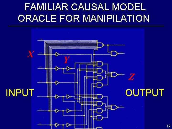
FAMILIAR CAUSAL MODEL ORACLE FOR MANIPILATION X Y Z INPUT OUTPUT 12

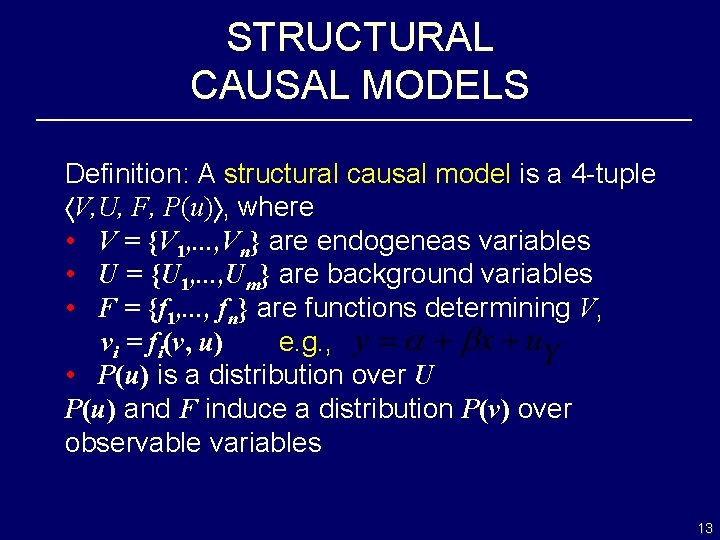
STRUCTURAL CAUSAL MODELS Definition: A structural causal model is a 4 -tuple V, U, F, P(u) , where • V = {V 1, . . . , Vn} are endogeneas variables • U = {U 1, . . . , Um} are background variables • F = {f 1, . . . , fn} are functions determining V, vi = fi(v, u) e. g. , • P(u) is a distribution over U P(u) and F induce a distribution P(v) over observable variables 13

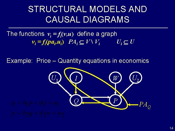
STRUCTURAL MODELS AND CAUSAL DIAGRAMS The functions vi = fi(v, u) define a graph vi = fi(pai, ui) PAi V Vi Ui U Example: Price – Quantity equations in economics U 1 I W Q P U 2 PAQ 14

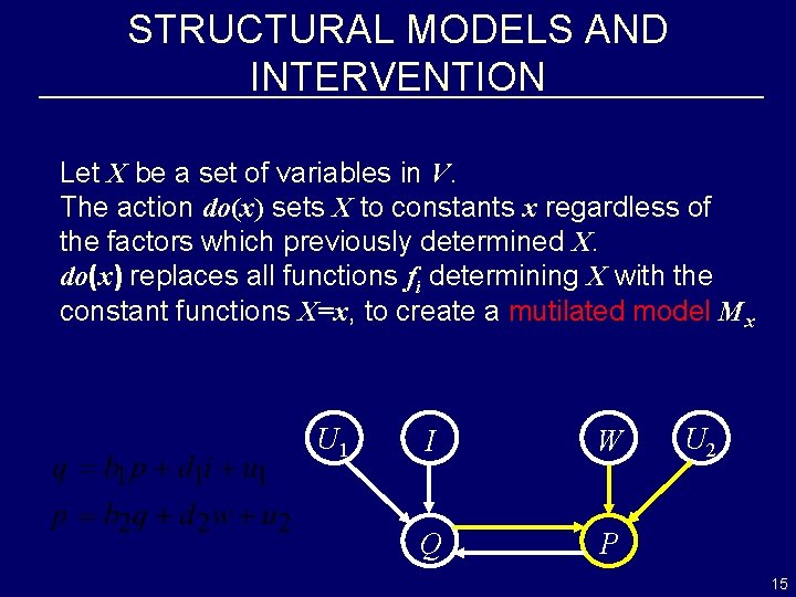
STRUCTURAL MODELS AND INTERVENTION Let X be a set of variables in V. The action do(x) sets X to constants x regardless of the factors which previously determined X. do(x) replaces all functions fi determining X with the constant functions X=x, to create a mutilated model Mx U 1 I W Q P U 2 15

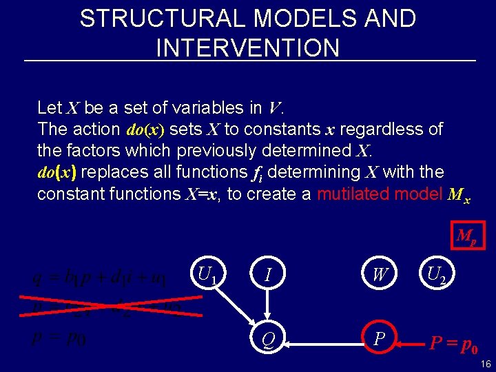
STRUCTURAL MODELS AND INTERVENTION Let X be a set of variables in V. The action do(x) sets X to constants x regardless of the factors which previously determined X. do(x) replaces all functions fi determining X with the constant functions X=x, to create a mutilated model Mx Mp U 1 I W U 2 Q P P = p 0 16

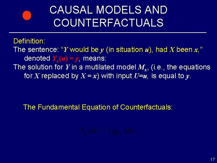
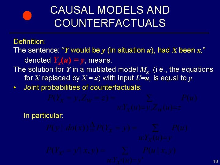
CAUSAL MODELS AND COUNTERFACTUALS Definition: The sentence: “Y would be y (in situation u), had X been x, ” denoted Yx(u) = y, means: The solution for Y in a mutilated model Mx, (i. e. , the equations for X replaced by X = x) with input U=u, is equal to y. The Fundamental Equation of Counterfactuals: 17

CAUSAL MODELS AND COUNTERFACTUALS Definition: The sentence: “Y would be y (in situation u), had X been x, ” denoted Yx(u) = y, means: The solution for Y in a mutilated model Mx, (i. e. , the equations for X replaced by X = x) with input U=u, is equal to y. • Joint probabilities of counterfactuals: In particular: 18

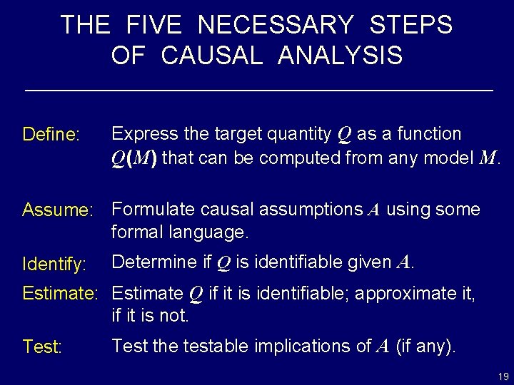
THE FIVE NECESSARY STEPS OF CAUSAL ANALYSIS Define: Express the target quantity Q as a function Q(M) that can be computed from any model M. Assume: Formulate causal assumptions A using some formal language. Identify: Determine if Q is identifiable given A. Estimate: Estimate Q if it is identifiable; approximate it, if it is not. Test: Test the testable implications of A (if any). 19

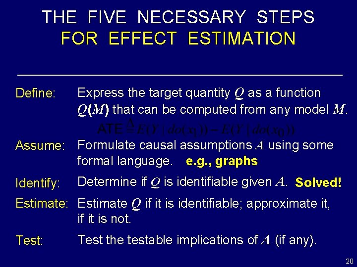
THE FIVE NECESSARY STEPS FOR EFFECT ESTIMATION Define: Express the target quantity Q as a function Q(M) that can be computed from any model M. Assume: Formulate causal assumptions A using some formal language. e. g. , graphs Identify: Determine if Q is identifiable given A. Solved! Estimate: Estimate Q if it is identifiable; approximate it, if it is not. Test: Test the testable implications of A (if any). 20

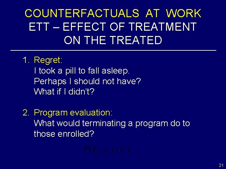
COUNTERFACTUALS AT WORK ETT – EFFECT OF TREATMENT ON THE TREATED 1. Regret: I took a pill to fall asleep. Perhaps I should not have? What if I didn’t? 2. Program evaluation: What would terminating a program do to those enrolled? 21

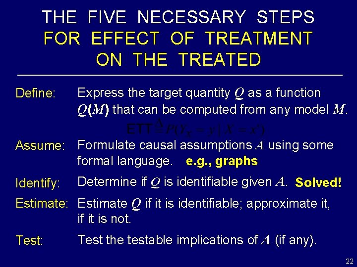
THE FIVE NECESSARY STEPS FOR EFFECT OF TREATMENT ON THE TREATED Define: Express the target quantity Q as a function Q(M) that can be computed from any model M. Assume: Formulate causal assumptions A using some formal language. e. g. , graphs Identify: Determine if Q is identifiable given A. Solved! Estimate: Estimate Q if it is identifiable; approximate it, if it is not. Test: Test the testable implications of A (if any). 22

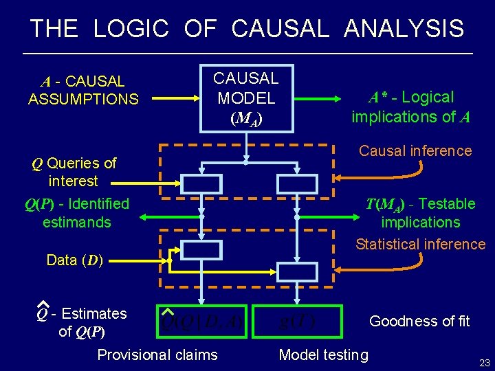
THE LOGIC OF CAUSAL ANALYSIS A - CAUSAL ASSUMPTIONS CAUSAL MODEL (MA) Q Queries of interest Q(P) - Identified estimands Data (D) A* - Logical implications of A Causal inference T(MA) - Testable implications Statistical inference Q - Estimates of Q(P) Provisional claims Goodness of fit Model testing 23

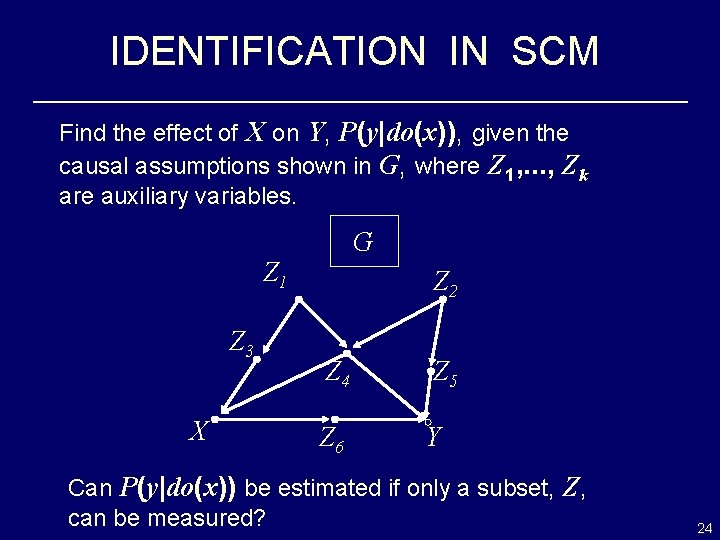
IDENTIFICATION IN SCM Find the effect of X on Y, P(y|do(x)), given the causal assumptions shown in G, where Z 1, . . . , Zk are auxiliary variables. G Z 1 Z 3 X Z 2 Z 4 Z 5 Z 6 Y Can P(y|do(x)) be estimated if only a subset, Z, can be measured? 24

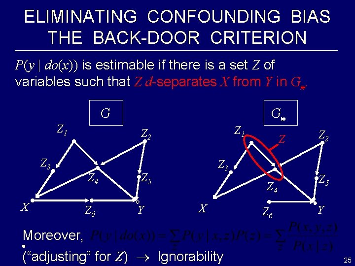
ELIMINATING CONFOUNDING BIAS THE BACK-DOOR CRITERION P(y | do(x)) is estimable if there is a set Z of variables such that Z d-separates X from Y in Gx. G Z 1 Z 3 X Gx Z 1 Z 2 Z 4 Z 6 Z 3 Z 5 Y Z Z 4 X Z 6 Z 2 Z 5 Y Moreover, • (“adjusting” for Z) Ignorability 25

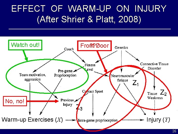
EFFECT OF WARM-UP ON INJURY (After Shrier & Platt, 2008) Watch out! ? ? ? Front Door No, no! Warm-up Exercises (X) Injury (Y) 26

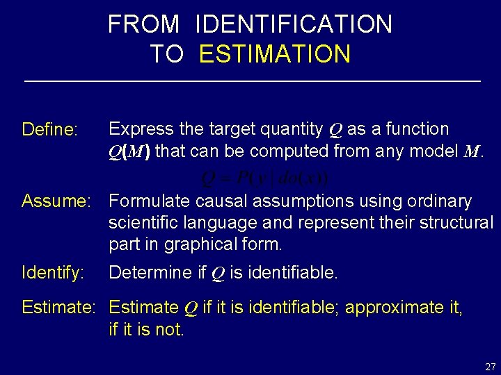
FROM IDENTIFICATION TO ESTIMATION Define: Express the target quantity Q as a function Q(M) that can be computed from any model M. Assume: Formulate causal assumptions using ordinary scientific language and represent their structural part in graphical form. Identify: Determine if Q is identifiable. Estimate: Estimate Q if it is identifiable; approximate it, if it is not. 27

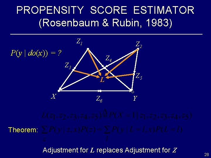
PROPENSITY SCORE ESTIMATOR (Rosenbaum & Rubin, 1983) Z 1 Z 2 P(y | do(x)) = ? Z 4 Z 3 L X Z 6 Z 5 Y Theorem: Adjustment for L replaces Adjustment for Z 28

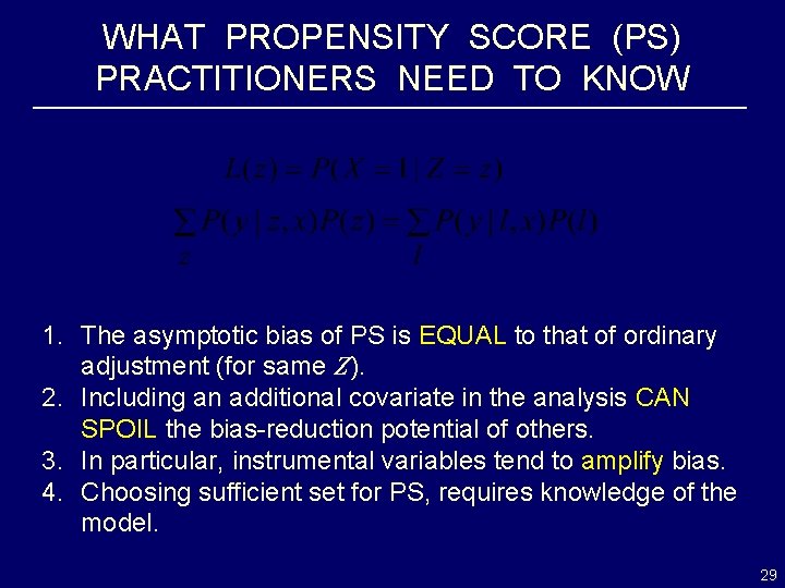
WHAT PROPENSITY SCORE (PS) PRACTITIONERS NEED TO KNOW 1. The asymptotic bias of PS is EQUAL to that of ordinary adjustment (for same Z). 2. Including an additional covariate in the analysis CAN SPOIL the bias-reduction potential of others. 3. In particular, instrumental variables tend to amplify bias. 4. Choosing sufficient set for PS, requires knowledge of the model. 29

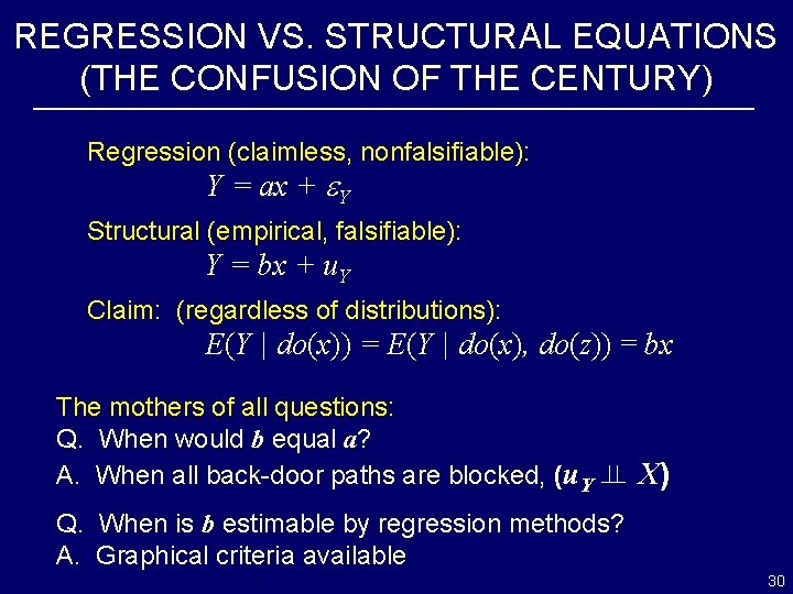
REGRESSION VS. STRUCTURAL EQUATIONS (THE CONFUSION OF THE CENTURY) Regression (claimless, nonfalsifiable): Y = ax + Y Structural (empirical, falsifiable): Y = bx + u. Y Claim: (regardless of distributions): E(Y | do(x)) = E(Y | do(x), do(z)) = bx The mothers of all questions: Q. When would b equal a? A. When all back-door paths are blocked, (u. Y X) Q. When is b estimable by regression methods? A. Graphical criteria available 30

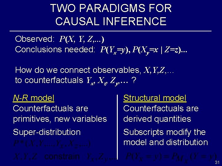
TWO PARADIGMS FOR CAUSAL INFERENCE Observed: P(X, Y, Z, . . . ) Conclusions needed: P(Yx=y), P(Xy=x | Z=z). . . How do we connect observables, X, Y, Z, … to counterfactuals Yx, Xz, Zy, … ? N-R model Counterfactuals are primitives, new variables Structural model Counterfactuals are derived quantities Super-distribution Subscripts modify the model and distribution 31

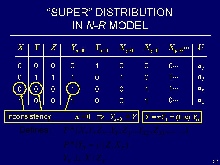
“SUPER” DISTRIBUTION IN N-R MODEL X Y Z Yx=0 Yx=1 Xz=0 Xz=1 Xy=0 U 0 0 1 0 0 0 1 1 1 0 0 1 u 2 0 0 0 1 1 u 3 1 0 0 1 0 u 4 inconsistency: x = 0 Yx=0 = Y Y = x. Y 1 + (1 -x) Y 0 32

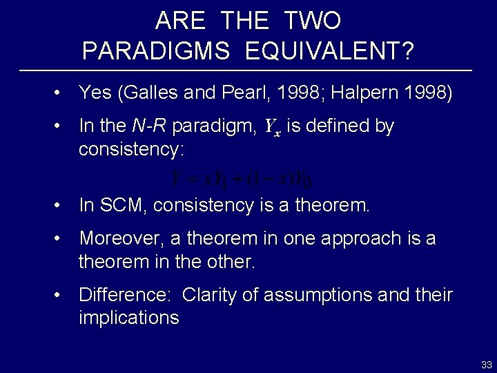
ARE THE TWO PARADIGMS EQUIVALENT? • Yes (Galles and Pearl, 1998; Halpern 1998) • In the N-R paradigm, Yx is defined by consistency: • In SCM, consistency is a theorem. • Moreover, a theorem in one approach is a theorem in the other. • Difference: Clarity of assumptions and their implications 33

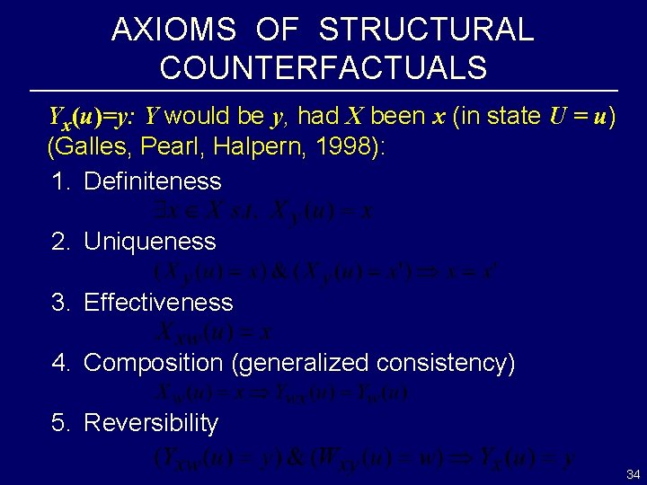
AXIOMS OF STRUCTURAL COUNTERFACTUALS Yx(u)=y: Y would be y, had X been x (in state U = u) (Galles, Pearl, Halpern, 1998): 1. Definiteness 2. Uniqueness 3. Effectiveness 4. Composition (generalized consistency) 5. Reversibility 34

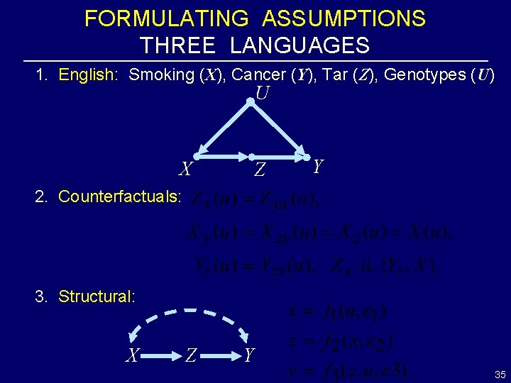
FORMULATING ASSUMPTIONS THREE LANGUAGES 1. English: Smoking (X), Cancer (Y), Tar (Z), Genotypes (U) U X Z Y 2. Counterfactuals: 3. Structural: X Z Y 35

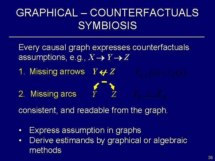
GRAPHICAL – COUNTERFACTUALS SYMBIOSIS Every causal graph expresses counterfactuals assumptions, e. g. , X Y Z 1. Missing arrows Y Z 2. Missing arcs Y Z consistent, and readable from the graph. • Express assumption in graphs • Derive estimands by graphical or algebraic methods 36

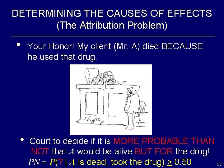
DETERMINING THE CAUSES OF EFFECTS (The Attribution Problem) • • Your Honor! My client (Mr. A) died BECAUSE he used that drug. Court to decide if it is MORE PROBABLE THAN NOT that A would be alive BUT FOR the drug! PN = P(? | A is dead, took the drug) > 0. 50 37

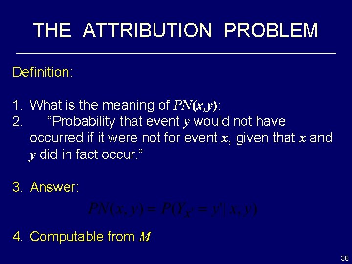
THE ATTRIBUTION PROBLEM Definition: 1. What is the meaning of PN(x, y): 2. “Probability that event y would not have occurred if it were not for event x, given that x and y did in fact occur. ” 3. Answer: 4. Computable from M 38

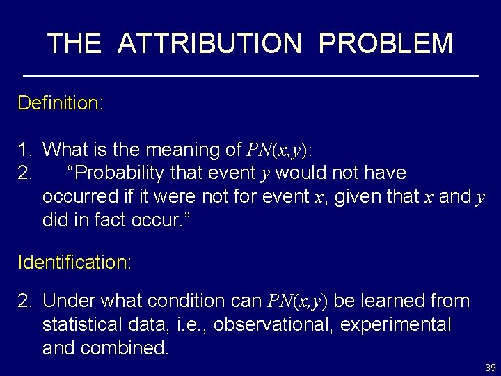
THE ATTRIBUTION PROBLEM Definition: 1. What is the meaning of PN(x, y): 2. “Probability that event y would not have occurred if it were not for event x, given that x and y did in fact occur. ” Identification: 2. Under what condition can PN(x, y) be learned from statistical data, i. e. , observational, experimental and combined. 39

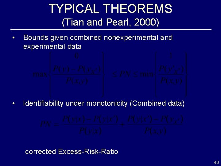
TYPICAL THEOREMS (Tian and Pearl, 2000) • Bounds given combined nonexperimental and experimental data • Identifiability under monotonicity (Combined data) corrected Excess-Risk-Ratio 40

CAN FREQUENCY DATA DECIDE LEGAL RESPONSIBILITY? Deaths (y) Survivals (y ) • • Experimental do(x) do(x ) 16 14 986 1, 000 Nonexperimental x x 2 28 998 972 1, 000 Nonexperimental data: drug usage predicts longer life Experimental data: drug has negligible effect on survival Plaintiff: Mr. A is special. 1. He actually died 2. He used the drug by choice Court to decide (given both data): Is it more probable than not that A would be alive but for the drug? 41

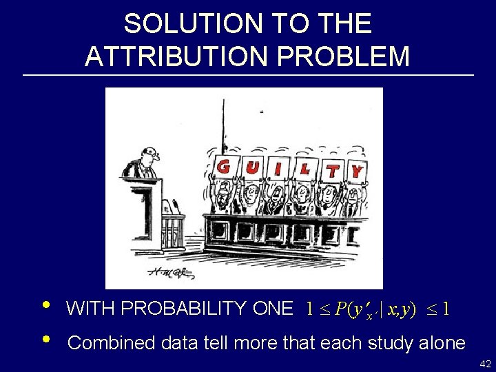
SOLUTION TO THE ATTRIBUTION PROBLEM • • WITH PROBABILITY ONE 1 P(y x | x, y) 1 Combined data tell more that each study alone 42

EFFECT DECOMPOSITION (direct vs. indirect effects) 1. Why decompose effects? 2. What is the definition of direct and indirect effects? 3. What are the policy implications of direct and indirect effects? 4. When can direct and indirect effect be estimated consistently from experimental and nonexperimental data? 43

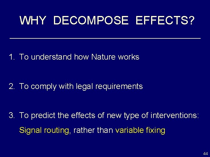
WHY DECOMPOSE EFFECTS? 1. To understand how Nature works 2. To comply with legal requirements 3. To predict the effects of new type of interventions: Signal routing, rather than variable fixing 44

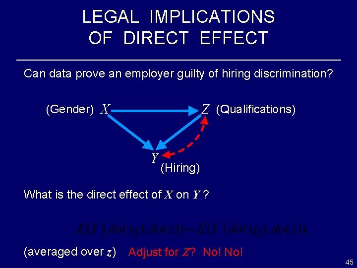
LEGAL IMPLICATIONS OF DIRECT EFFECT Can data prove an employer guilty of hiring discrimination? (Gender) X Z (Qualifications) Y (Hiring) What is the direct effect of X on Y ? (averaged over z) Adjust for Z? No! 45

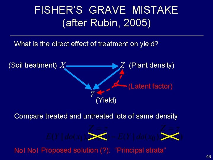
FISHER’S GRAVE MISTAKE (after Rubin, 2005) What is the direct effect of treatment on yield? (Soil treatment) X Z (Plant density) Y (Latent factor) (Yield) Compare treated and untreated lots of same density No! Proposed solution (? ): “Principal strata” 46

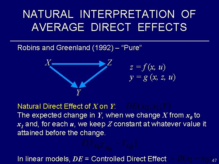
NATURAL INTERPRETATION OF AVERAGE DIRECT EFFECTS Robins and Greenland (1992) – “Pure” X Z z = f (x, u) y = g (x, z, u) Y Natural Direct Effect of X on Y: The expected change in Y, when we change X from x 0 to x 1 and, for each u, we keep Z constant at whatever value it attained before the change. In linear models, DE = Controlled Direct Effect 47

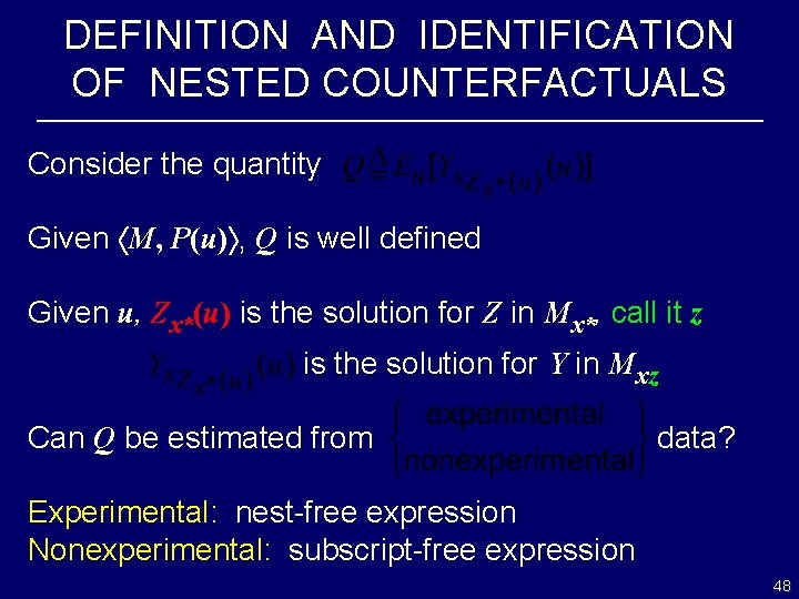
DEFINITION AND IDENTIFICATION OF NESTED COUNTERFACTUALS Consider the quantity Given M, P(u) , Q is well defined Given u, Zx*(u) is the solution for Z in Mx*, call it z is the solution for Y in Mxz Can Q be estimated from data? Experimental: nest-free expression Nonexperimental: subscript-free expression 48

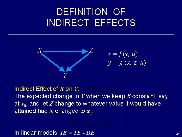
DEFINITION OF INDIRECT EFFECTS X Z z = f (x, u) y = g (x, z, u) Y Indirect Effect of X on Y: The expected change in Y when we keep X constant, say at x 0, and let Z change to whatever value it would have attained had X changed to x 1. In linear models, IE = TE - DE 49

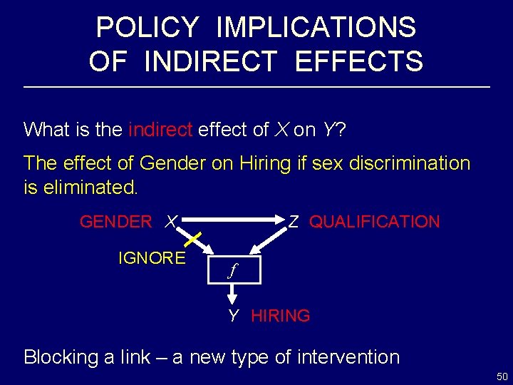
POLICY IMPLICATIONS OF INDIRECT EFFECTS What is the indirect effect of X on Y? The effect of Gender on Hiring if sex discrimination is eliminated. GENDER X IGNORE Z QUALIFICATION f Y HIRING Blocking a link – a new type of intervention 50

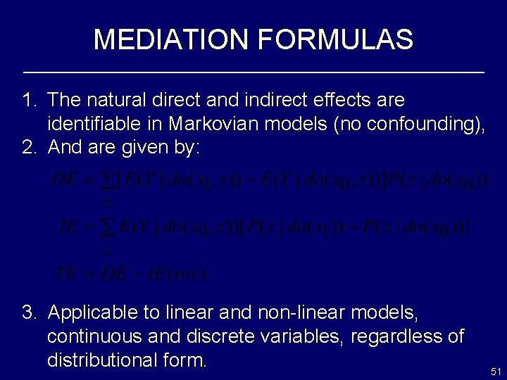
MEDIATION FORMULAS 1. The natural direct and indirect effects are identifiable in Markovian models (no confounding), 2. And are given by: 3. Applicable to linear and non-linear models, continuous and discrete variables, regardless of distributional form. 51

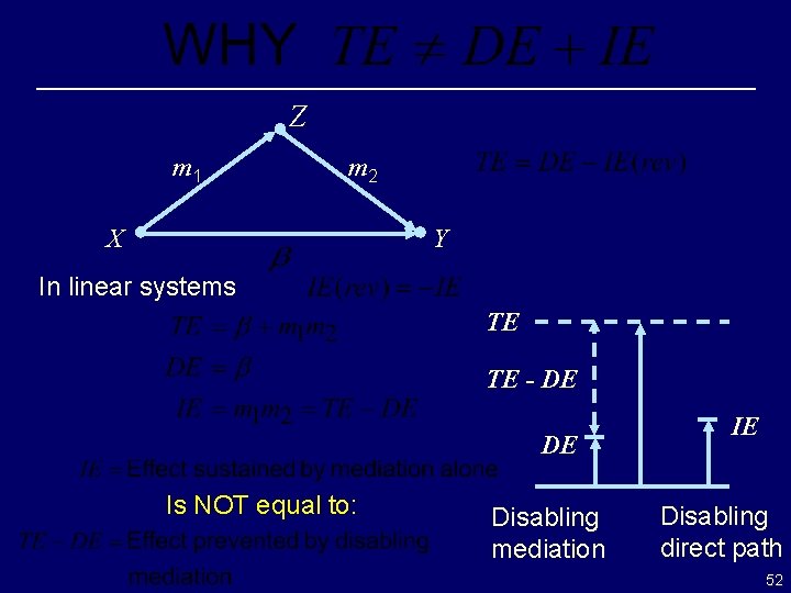
Z m 1 m 2 X Y In linear systems TE TE - DE DE Is NOT equal to: Disabling mediation IE Disabling direct path 52

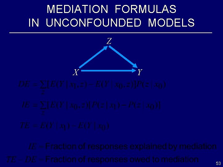
MEDIATION FORMULAS IN UNCONFOUNDED MODELS Z X Y 53

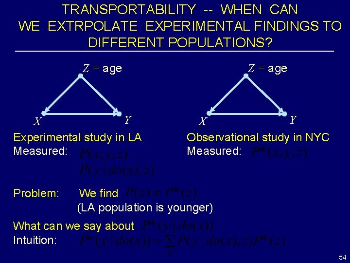
TRANSPORTABILITY -- WHEN CAN WE EXTRPOLATE EXPERIMENTAL FINDINGS TO DIFFERENT POPULATIONS? Z = age Y X Experimental study in LA Measured: Problem: Z = age Y X Observational study in NYC Measured: We find (LA population is younger) What can we say about Intuition: 54

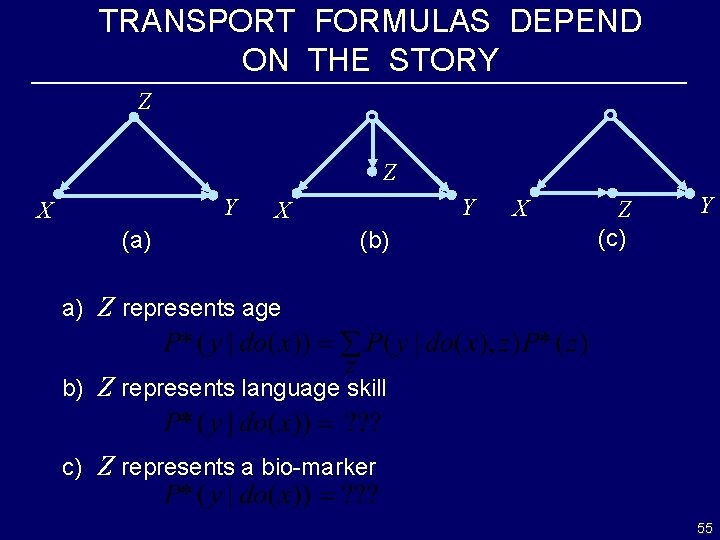
TRANSPORT FORMULAS DEPEND ON THE STORY Z Z Y X (a) (b) X Z (c) Y a) Z represents age b) Z represents language skill c) Z represents a bio-marker 55

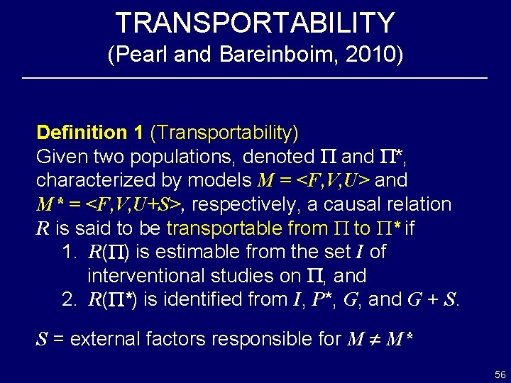
TRANSPORTABILITY (Pearl and Bareinboim, 2010) Definition 1 (Transportability) Given two populations, denoted and *, characterized by models M = <F, V, U> and M* = <F, V, U+S>, respectively, a causal relation R is said to be transportable from to * if 1. R( ) is estimable from the set I of interventional studies on , and 2. R( *) is identified from I, P*, G, and G + S. S = external factors responsible for M M* 56

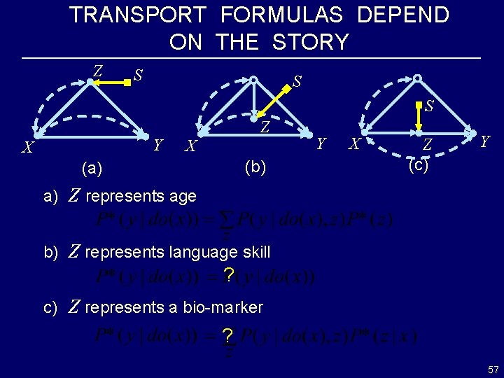
TRANSPORT FORMULAS DEPEND ON THE STORY Z S S S Y X Z X (b) (a) Y X Z (c) Y a) Z represents age b) Z represents language skill ? c) Z represents a bio-marker ? 57

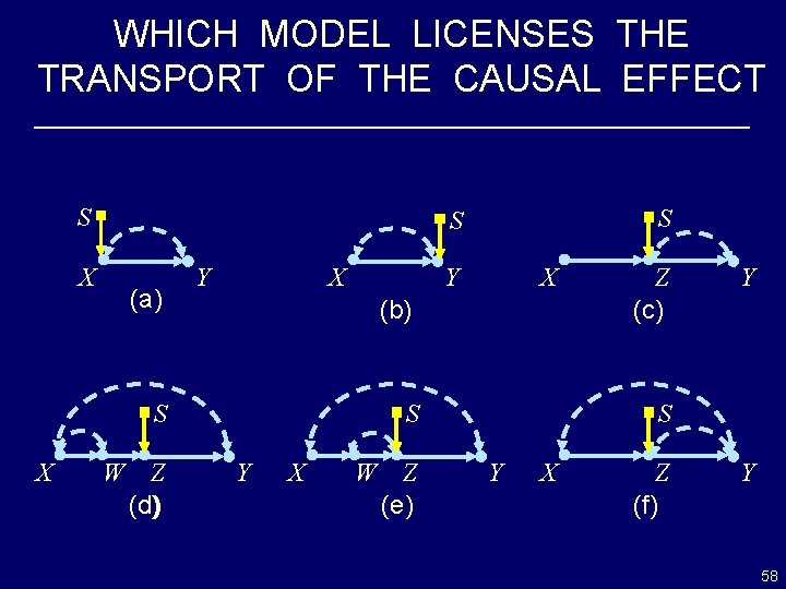
WHICH MODEL LICENSES THE TRANSPORT OF THE CAUSAL EFFECT S X (a) X Y W Z (c) (d) Y X (b) S X S S X W Z (e) Y S S Y Z (c) Y X Z ( (f) (f Y 58

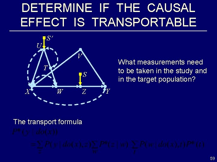
DETERMINE IF THE CAUSAL EFFECT IS TRANSPORTABLE U S V T X What measurements need to be taken in the study and in the target population? S W Z Y The transport formula 59

CONCLUSIONS I TOLD YOU CAUSALITY IS SIMPLE • Formal basis for causal and counterfactual inference (complete) • Unification of the graphical, potential-outcome and structural equation approaches • Friendly and formal solutions to century-old problems and confusions. • No other method can do better (theorem) 60

Thank you for agreeing with everything I said. 61