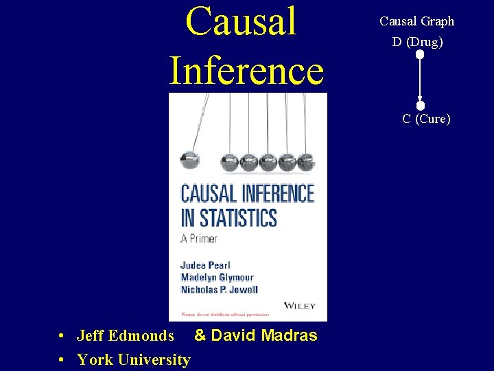
Causal Inference Causal Graph D Drug C Cure

Causal Inference Causal Graph D (Drug) C (Cure) • Jeff Edmonds & David Madras • York University

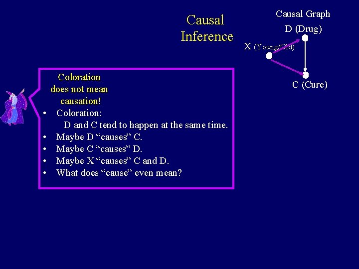
Causal Inference • • • Coloration does not mean causation! Coloration: D and C tend to happen at the same time. Maybe D “causes” C. Maybe C “causes” D. Maybe X “causes” C and D. What does “cause” even mean? Causal Graph D (Drug) X (Young/Old) C (Cure)

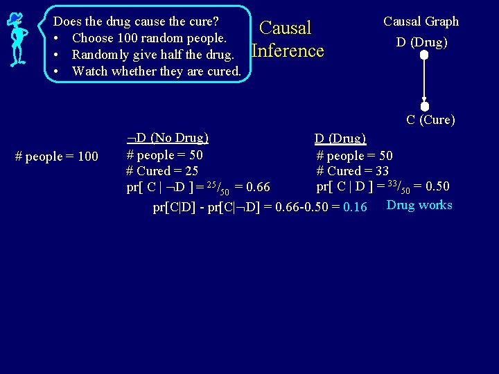
Does the drug cause the cure? • Choose 100 random people. • Randomly give half the drug. • Watch whether they are cured. Causal Inference Causal Graph D (Drug) C (Cure) # people = 100 D (No Drug) D (Drug) # people = 50 # Cured = 25 # Cured = 33 pr[ C | D ] = 33/50 = 0. 50 pr[ C | D ] = 25/50 = 0. 66 pr[C|D] - pr[C| D] = 0. 66 -0. 50 = 0. 16 Drug works

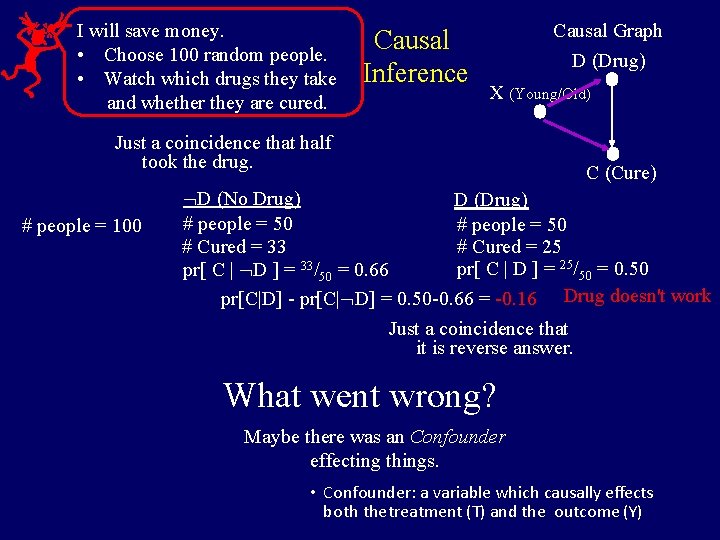
I will save money. • Choose 100 random people. • Watch which drugs they take and whether they are cured. Causal Inference Causal Graph D (Drug) X (Young/Old) Just a coincidence that half took the drug. # people = 100 C (Cure) D (No Drug) D (Drug) # people = 50 # Cured = 33 # Cured = 25 pr[ C | D ] = 25/50 = 0. 50 pr[ C | D ] = 33/50 = 0. 66 pr[C|D] - pr[C| D] = 0. 50 -0. 66 = -0. 16 Drug doesn't work Just a coincidence that it is reverse answer. What went wrong? Maybe there was an Confounder effecting things. • Confounder: a variable which causally effects both the treatment (T) and the outcome (Y)

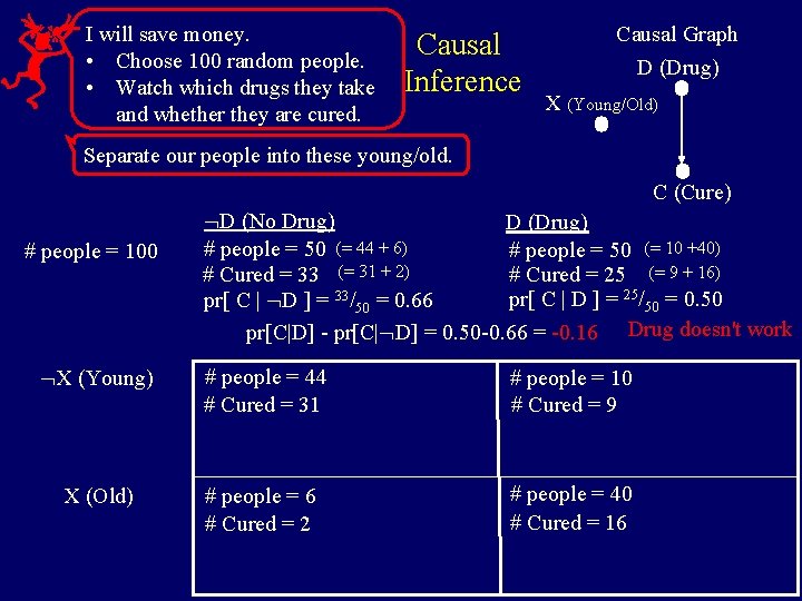
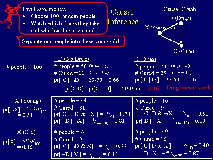
I will save money. • Choose 100 random people. • Watch which drugs they take and whether they are cured. Causal Inference Causal Graph D (Drug) X (Young/Old) Separate our people into these young/old. C (Cure) # people = 100 D (No Drug) D (Drug) # people = 50 (= 44 + 6) # people = 50 (= 10 +40) # Cured = 33 (= 31 + 2) # Cured = 25 (= 9 + 16) pr[ C | D ] = 25/50 = 0. 50 pr[ C | D ] = 33/50 = 0. 66 pr[C|D] - pr[C| D] = 0. 50 -0. 66 = -0. 16 Drug doesn't work X (Young) # people = 44 # Cured = 31 # people = 10 # Cured = 9 X (Old) # people = 6 # Cured = 2 # people = 40 # Cured = 16

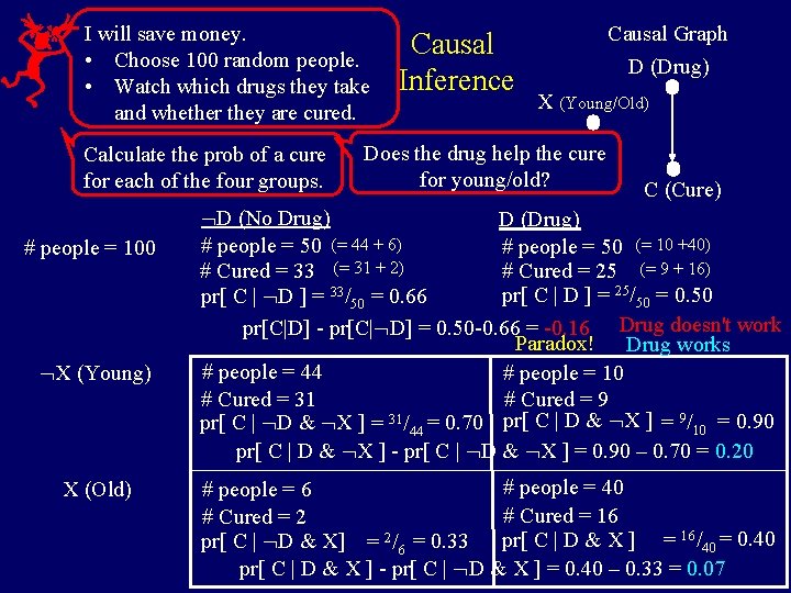
I will save money. • Choose 100 random people. • Watch which drugs they take and whether they are cured. Calculate the prob of a cure for each of the four groups. # people = 100 X (Young) X (Old) Causal Inference Causal Graph D (Drug) X (Young/Old) Does the drug help the cure for young/old? C (Cure) D (No Drug) D (Drug) # people = 50 (= 44 + 6) # people = 50 (= 10 +40) # Cured = 33 (= 31 + 2) # Cured = 25 (= 9 + 16) pr[ C | D ] = 25/50 = 0. 50 pr[ C | D ] = 33/50 = 0. 66 pr[C|D] - pr[C| D] = 0. 50 -0. 66 = -0. 16 Drug doesn't work Paradox! Drug works # people = 44 # people = 10 # Cured = 31 # Cured = 9 pr[ C | D & X ] = 31/44 = 0. 70 pr[ C | D & X ] = 9/10 = 0. 90 pr[ C | D & X ] - pr[ C | D & X ] = 0. 90 – 0. 70 = 0. 20 # people = 40 # people = 6 # Cured = 16 # Cured = 2 pr[ C | D & X] = 2/6 = 0. 33 pr[ C | D & X ] = 16/40 = 0. 40 pr[ C | D & X ] - pr[ C | D & X ] = 0. 40 – 0. 33 = 0. 07

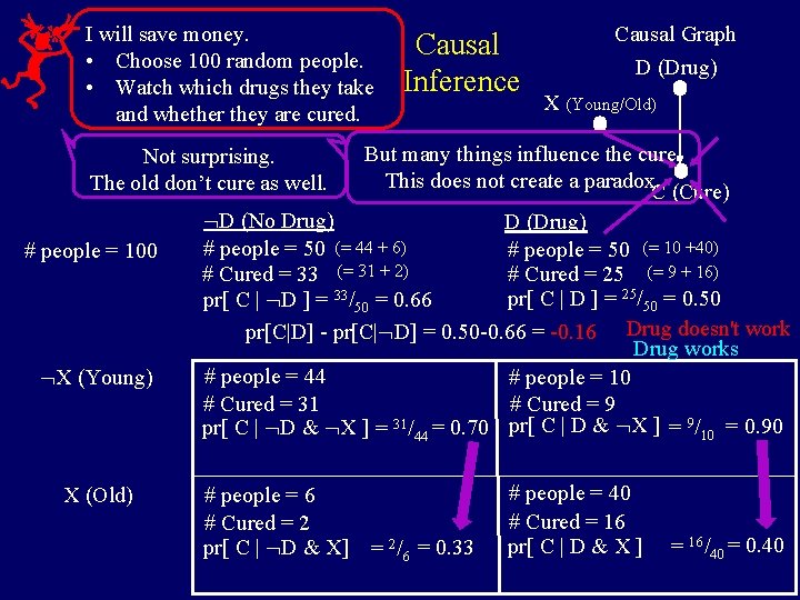
I will save money. • Choose 100 random people. • Watch which drugs they take and whether they are cured. Causal Inference Causal Graph D (Drug) X (Young/Old) But many things influence the cure. This does not create a paradox. C (Cure) D (No Drug) D (Drug) # people = 50 (= 44 + 6) # people = 50 (= 10 +40) # Cured = 33 (= 31 + 2) # Cured = 25 (= 9 + 16) pr[ C | D ] = 25/50 = 0. 50 pr[ C | D ] = 33/50 = 0. 66 pr[C|D] - pr[C| D] = 0. 50 -0. 66 = -0. 16 Drug doesn't work Drug works # people = 44 # people = 10 # Cured = 31 # Cured = 9 pr[ C | D & X ] = 31/44 = 0. 70 pr[ C | D & X ] = 9/10 = 0. 90 Not surprising. The old don’t cure as well. # people = 100 X (Young) X (Old) # people = 6 # Cured = 2 pr[ C | D & X] = 2/6 = 0. 33 # people = 40 # Cured = 16 pr[ C | D & X ] = 16/40 = 0. 40

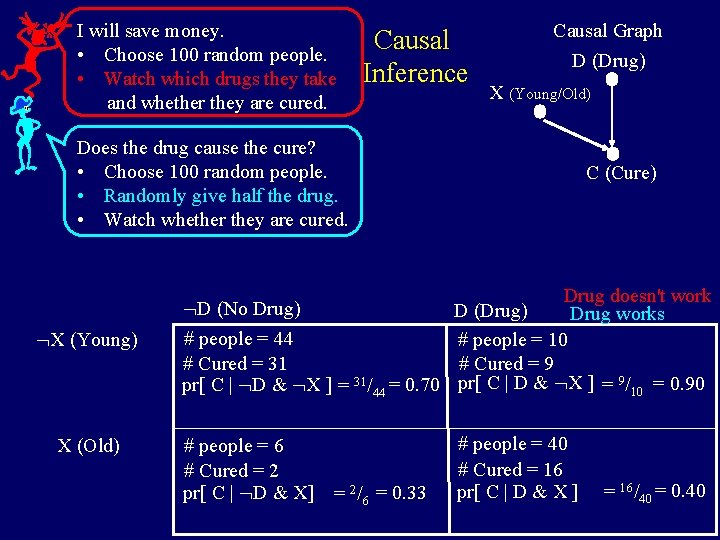
I will save money. • Choose 100 random people. • Watch which drugs they take and whether they are cured. Causal Inference Causal Graph D (Drug) X (Young/Old) Does the drug cause the cure? • Choose 100 random people. • Randomly give half the drug. • Watch whether they are cured. X (Young) X (Old) C (Cure) D (No Drug) # people = 44 # Cured = 31 pr[ C | D & X ] = 31/44 = 0. 70 Drug doesn't work D (Drug) Drug works # people = 10 # Cured = 9 pr[ C | D & X ] = 9/10 = 0. 90 # people = 6 # Cured = 2 pr[ C | D & X] = 2/6 = 0. 33 # people = 40 # Cured = 16 pr[ C | D & X ] = 16/40 = 0. 40

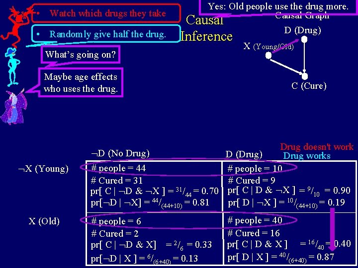
• Watch which drugs they take • Randomly give half the drug. Yes: Old people use the drug more. Causal Graph Causal Inference What’s going on? Maybe age effects who uses the drug. X (Young) X (Old) D (Drug) X (Young/Old) C (Cure) D (No Drug) # people = 44 # Cured = 31 pr[ C | D & X ] = 31/44 = 0. 70 pr[ D | X] = 44/(44+10) = 0. 81 Drug doesn't work D (Drug) Drug works # people = 10 # Cured = 9 pr[ C | D & X ] = 9/10 = 0. 90 pr[ D | X ] = 10/(44+10) = 0. 19 # people = 6 # Cured = 2 pr[ C | D & X] = 2/6 = 0. 33 pr[ D | X ] = 6/(6+40) = 0. 13 # people = 40 # Cured = 16 pr[ C | D & X ] = 16/40 = 0. 40 pr[ D | X ] = 40/(6+40) = 0. 87

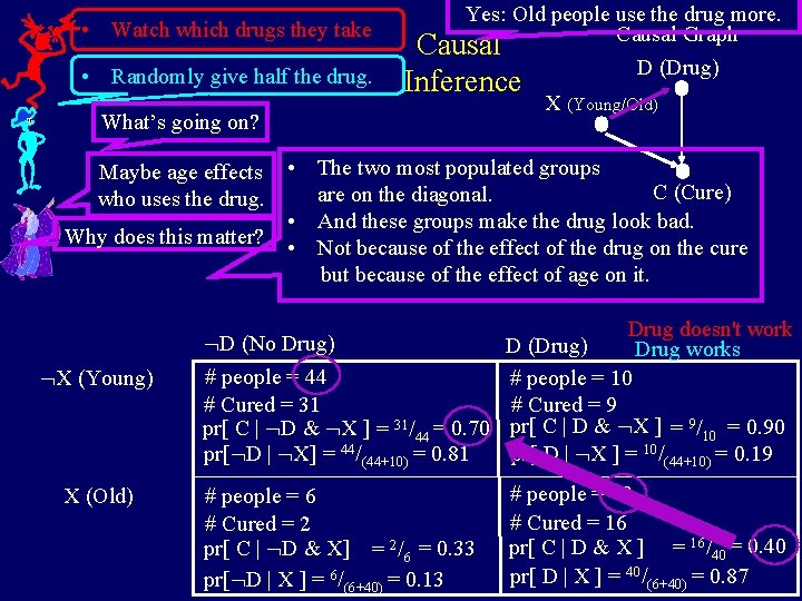
• Watch which drugs they take • Randomly give half the drug. Yes: Old people use the drug more. Causal Graph Causal Inference What’s going on? Maybe age effects who uses the drug. Why does this matter? X (Young) X (Old) D (Drug) X (Young/Old) • The two most populated groups C (Cure) are on the diagonal. • And these groups make the drug look bad. • Not because of the effect of the drug on the cure but because of the effect of age on it. D (No Drug) # people = 44 # Cured = 31 pr[ C | D & X ] = 31/44 = 0. 70 pr[ D | X] = 44/(44+10) = 0. 81 Drug doesn't work D (Drug) Drug works # people = 10 # Cured = 9 pr[ C | D & X ] = 9/10 = 0. 90 pr[ D | X ] = 10/(44+10) = 0. 19 # people = 6 # Cured = 2 pr[ C | D & X] = 2/6 = 0. 33 pr[ D | X ] = 6/(6+40) = 0. 13 # people = 40 # Cured = 16 pr[ C | D & X ] = 16/40 = 0. 40 pr[ D | X ] = 40/(6+40) = 0. 87

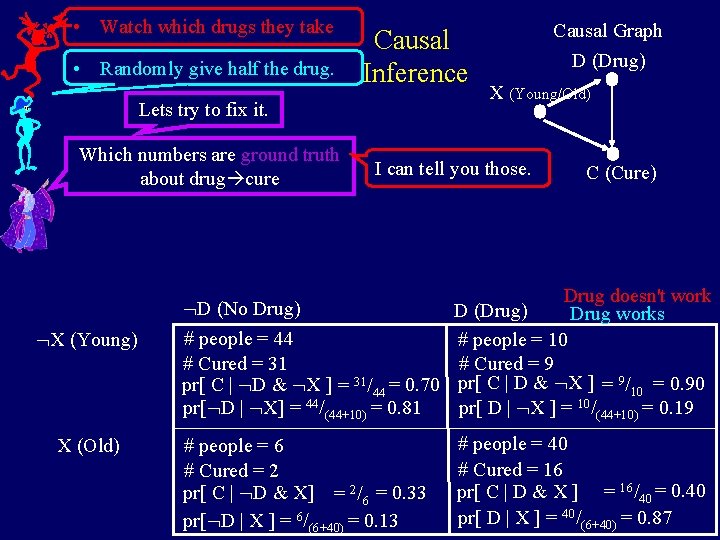
• Watch which drugs they take • Randomly give half the drug. Causal Inference Lets try to fix it. Which numbers are ground truth about drug cure X (Young) X (Old) Causal Graph D (Drug) X (Young/Old) I can tell you those. C (Cure) D (No Drug) # people = 44 # Cured = 31 pr[ C | D & X ] = 31/44 = 0. 70 pr[ D | X] = 44/(44+10) = 0. 81 Drug doesn't work D (Drug) Drug works # people = 10 # Cured = 9 pr[ C | D & X ] = 9/10 = 0. 90 pr[ D | X ] = 10/(44+10) = 0. 19 # people = 6 # Cured = 2 pr[ C | D & X] = 2/6 = 0. 33 pr[ D | X ] = 6/(6+40) = 0. 13 # people = 40 # Cured = 16 pr[ C | D & X ] = 16/40 = 0. 40 pr[ D | X ] = 40/(6+40) = 0. 87

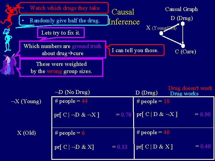
• Watch which drugs they take • Randomly give half the drug. Causal Inference Lets try to fix it. Which numbers are ground truth about drug cure Causal Graph D (Drug) X (Young/Old) I can tell you those. C (Cure) These were weighted by the wrong group sizes. X (Young) pr[ C | D & X ] X (Old) Drug doesn't work D (Drug) Drug works # people = 10 D (No Drug) # people = 44 = 0. 70 pr[ C | D & X ] # people = 40 # people = 6 pr[ C | D & X] = 0. 90 = 0. 33 pr[ C | D & X ] = 0. 40

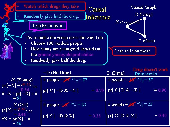
• Watch which drugs they take • Randomly give half the drug. Causal Inference Lets try to fix it. Try to make the group sizes the way I do. • Choose 100 random people. • How many are young/old depends on the ground young/old probabilies. • Randomly give half the drug. X (Young) pr[ X] = (44+10)/100 = 0. 54 # X = pr[ X] # = 54 X (Old) pr[X] = (6+40)/100 = 0. 46 #X = pr[X] # = 46 pr[ C | D & X] 2= X (Young/Old) C (Cure) I can tell you those. = 0. 70 pr[ C | D & X ] 46/ D (Drug) Drug doesn't work D (Drug) Drug works # people = 10 54/2 = 27 D (No Drug) # people = 44 54/2 = 27 # people = 6 Causal Graph # people = 40 23 = 0. 33 pr[ C | D & X ] 46/ = 0. 90 2= 23 = 0. 40

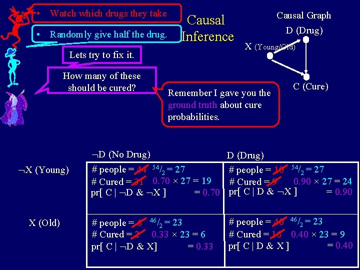
• Watch which drugs they take • Randomly give half the drug. Causal Inference Lets try to fix it. How many of these should be cured? X (Young) X (Old) Causal Graph D (Drug) X (Young/Old) Remember I gave you the ground truth about cure probabilities. C (Cure) D (No Drug) # people = 44 54/2 = 27 # Cured = 31 0. 70 × 27 = 19 pr[ C | D & X ] = 0. 70 D (Drug) # people = 10 54/2 = 27 0. 90 × 27 = 24 # Cured = 9 pr[ C | D & X ] = 0. 90 # people = 6 46/2 = 23 # Cured = 2 0. 33 × 23 = 6 pr[ C | D & X] = 0. 33 # people = 40 46/2 = 23 # Cured = 16 0. 40 × 23 = 9 = 0. 40 pr[ C | D & X ]

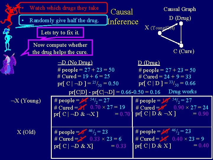
• Watch which drugs they take • Randomly give half the drug. Causal Inference Lets try to fix it. Now compute whether the drug helps the cure. X (Young) X (Old) Causal Graph D (Drug) X (Young/Old) C (Cure) D (No Drug) D (Drug) # people = 27 + 23 = 50 # Cured = 19 + 6 = 25 # Cured = 24 + 9 = 33 pr[ C | D ] = 33/50 = 0. 66 pr[ C | D ] = 25/50 = 0. 50 pr[C|D] - pr[C| D] = 0. 66 -0. 50 = 0. 16 Drug works # people = 44 54/2 = 27 # people = 10 54/2 = 27 0. 90 × 27 = 24 # Cured = 31 0. 70 × 27 = 19 # Cured = 9 = 0. 90 pr[ C | D & X ] = 0. 70 pr[ C | D & X ] # people = 6 46/2 = 23 # Cured = 2 0. 33 × 23 = 6 pr[ C | D & X] = 0. 33 # people = 40 46/2 = 23 # Cured = 16 0. 40 × 23 = 9 = 0. 40 pr[ C | D & X ]

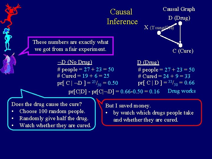
Causal Inference These numbers are exactly what we got from a fair experiment. Causal Graph D (Drug) X (Young/Old) C (Cure) D (No Drug) D (Drug) # people = 27 + 23 = 50 # Cured = 19 + 6 = 25 # Cured = 24 + 9 = 33 pr[ C | D ] = 33/50 = 0. 66 pr[ C | D ] = 25/50 = 0. 50 pr[C|D] - pr[C| D] = 0. 66 -0. 50 = 0. 16 Drug works Does the drug cause the cure? • Choose 100 random people. • Randomly give half the drug. • Watch whether they are cured. But I saved money. • by watch which drugs people take and whether they are cured.

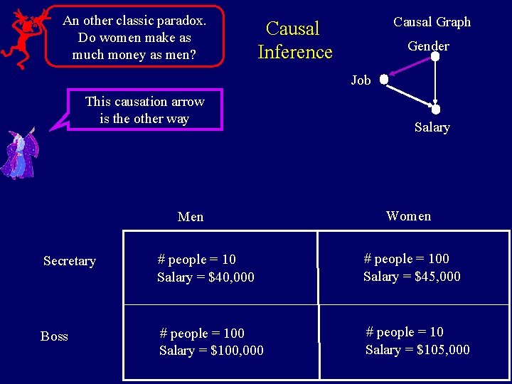
An other classic paradox. Do women make as much money as men? Causal Graph Causal Inference Gender Job This causation arrow is the other way Men Salary Women Secretary # people = 10 Salary = $40, 000 # people = 100 Salary = $45, 000 Boss # people = 100 Salary = $100, 000 # people = 10 Salary = $105, 000

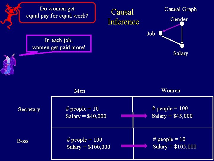
Do women get equal pay for equal work? Causal Graph Causal Inference Gender Job In each job, women get paid more! Men Salary Women Secretary # people = 10 Salary = $40, 000 # people = 100 Salary = $45, 000 Boss # people = 100 Salary = $100, 000 # people = 10 Salary = $105, 000

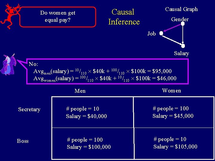
Do women get equal pay? Causal Graph Causal Inference Gender Job Salary No: Avgmen(salary) = 10/110 $40 k + 100/110 $100 k = $95, 000 Avgwomen(salary) = 100/110 $40 k + 10/110 $100 k = $46, 000 Men Women Secretary # people = 10 Salary = $40, 000 # people = 100 Salary = $45, 000 Boss # people = 100 Salary = $100, 000 # people = 10 Salary = $105, 000

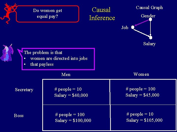
Do women get equal pay? Causal Graph Causal Inference Gender Job Salary The problem is that • women are directed into jobs • that payless Men Women Secretary # people = 10 Salary = $40, 000 # people = 100 Salary = $45, 000 Boss # people = 100 Salary = $100, 000 # people = 10 Salary = $105, 000

Intro to Causality David Madras October 22, 2019

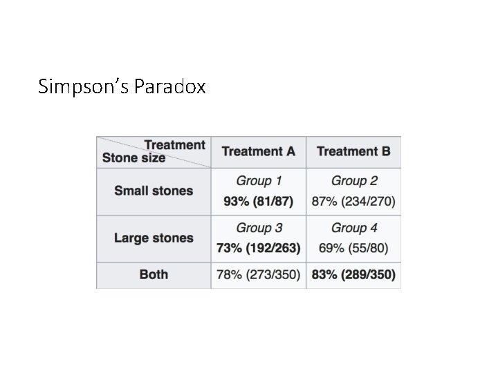
Simpson’s Paradox

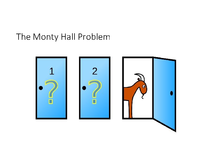
The Monty Hall Problem

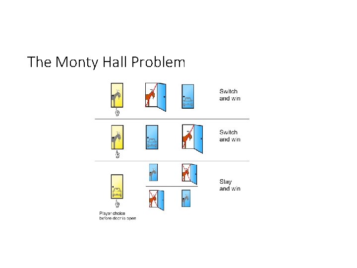
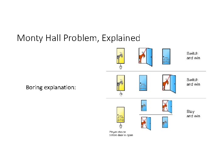
The Monty Hall Problem 1. Three doors – 2 have goats behind them, 1 has a car (you want to win the car) 2. You choose a door, but don’t open it 3. The host, Monty, opens another door (not the one you chose), and shows you that there is a goat behind that door 4. You now have the option to switch your door from the one you chose to the other unopened door 5. What should you do? Should you switch?

The Monty Hall Problem

What’s Going On?

Causation != Correlation • In machine learning, we try to learn correlations from data • “When can we predict X from Y? ” • In causal inference, we try to model causation • “When does X cause Y? ” • These are not the same! • Ice cream consumption correlates with murder rates • Ice cream does not cause murder (usually)

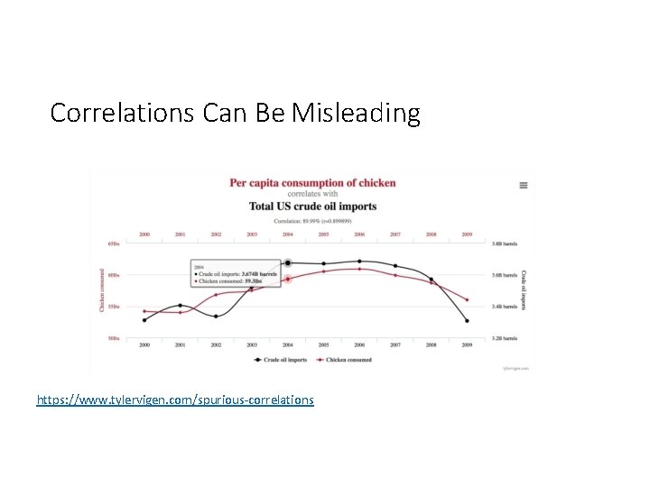
Correlations Can Be Misleading https: //www. tylervigen. com/spurious-correlations

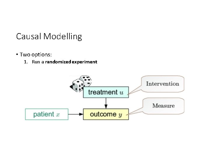
Causal Modelling • Two options: 1. Run a randomized experiment

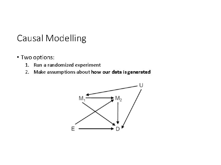
Causal Modelling • Two options: 1. Run a randomized experiment 2. Make assumptions about how our data is generated

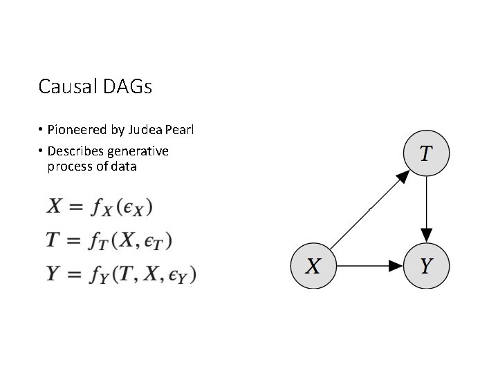
Causal DAGs • Pioneered by Judea Pearl • Describes generative process of data

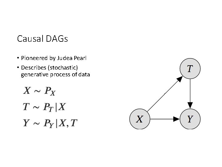
Causal DAGs • Pioneered by Judea Pearl • Describes (stochastic) generative process of data

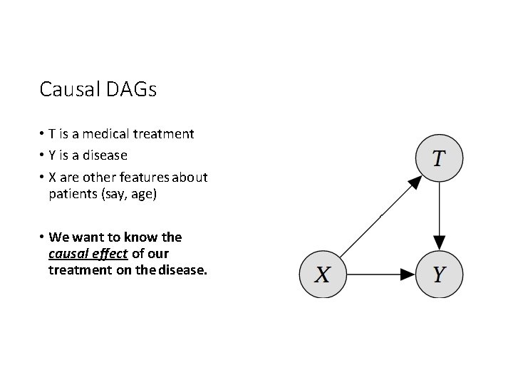
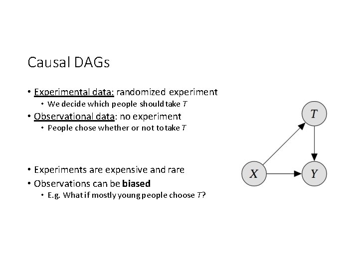
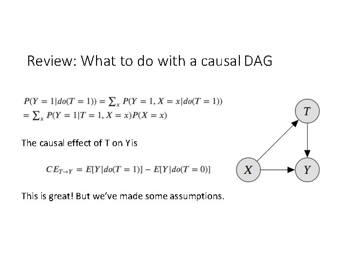
Causal DAGs • T is a medical treatment • Y is a disease • X are other features about patients (say, age) • We want to know the causal effect of our treatment on the disease.

Causal DAGs • Experimental data: randomized experiment • We decide which people should take T • Observational data: no experiment • People chose whether or not to take T • Experiments are expensive and rare • Observations can be biased • E. g. What if mostly young people choose T?

Asking Causal Questions • Suppose T is binary (1: received treatment, 0: did not) • Suppose Y is binary (1: disease cured, 0: disease not cured) • We want to know “If we give someone the treatment (T = 1), what is the probability they are cured (Y = 1)? ” • This is not equal to P(Y = 1 | T = 1) • Suppose mostly young people take the treatment, and most were cured, i. e. P(Y = 1 | T = 1) is high • Is this because the treatment is good? Or because they are young?

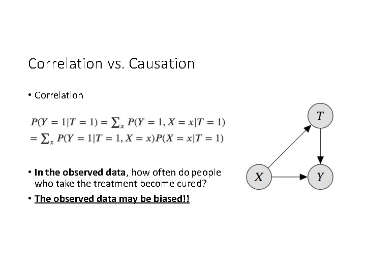
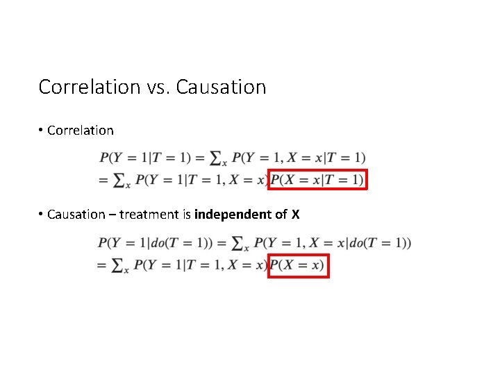
Correlation vs. Causation • Correlation • In the observed data, how often do people who take the treatment become cured? • The observed data may be biased!!

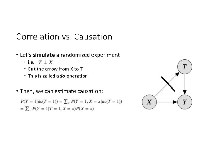
Correlation vs. Causation • Let’s simulate a randomized experiment • i. e. • Cut the arrow from X to T • This is called a do-operation • Then, we can estimate causation:

Correlation vs. Causation • Correlation • Causation – treatment is independent of X

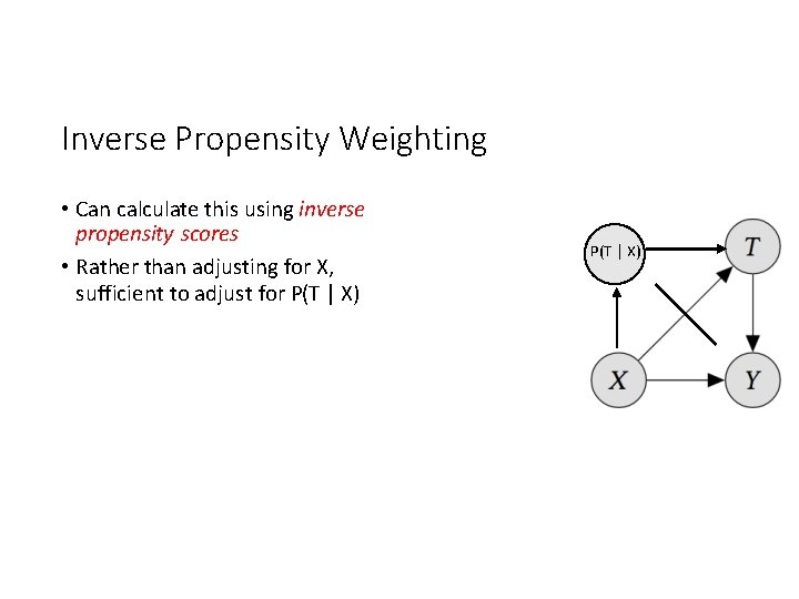
Inverse Propensity Weighting • Can calculate this using inverse propensity scores • Rather than adjusting for X, sufficient to adjust for P(T | X)

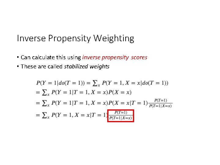
Inverse Propensity Weighting • Can calculate this using inverse propensity scores • These are called stabilized weights

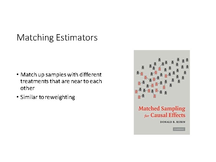
Matching Estimators • Match up samples with different treatments that are near to each other • Similar to reweighting

Review: What to do with a causal DAG The causal effect of T on Y is This is great! But we’ve made some assumptions.

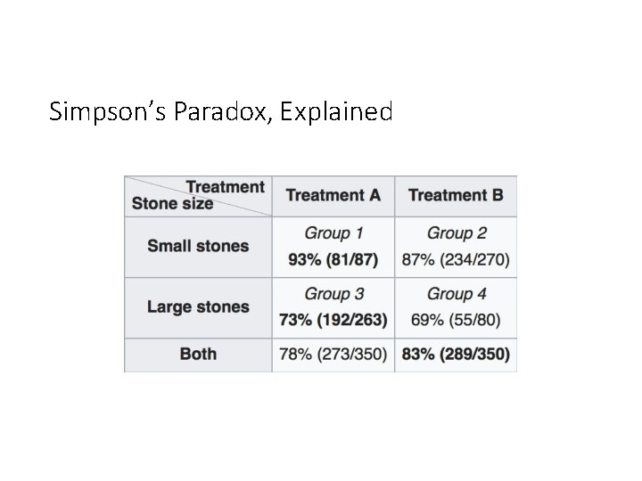
Simpson’s Paradox, Explained

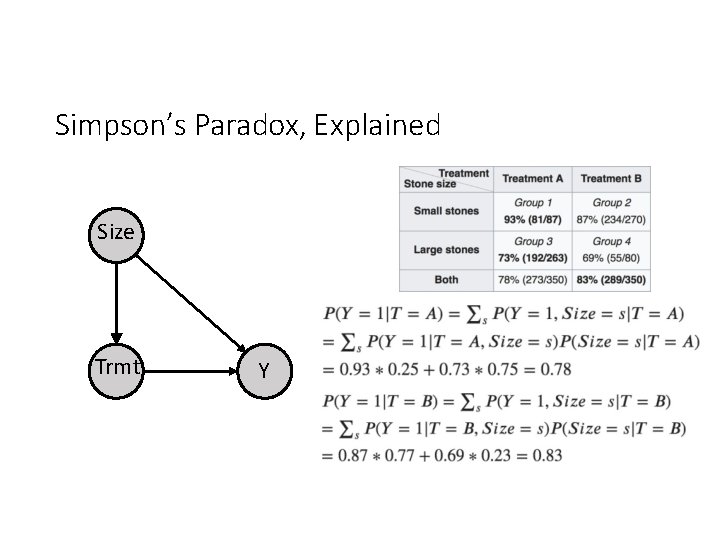
Simpson’s Paradox, Explained Size Trmt Y

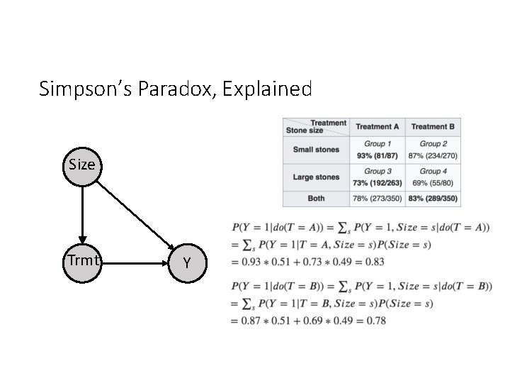
Simpson’s Paradox, Explained Size Trmt Y

Monty Hall Problem, Explained Boring explanation:

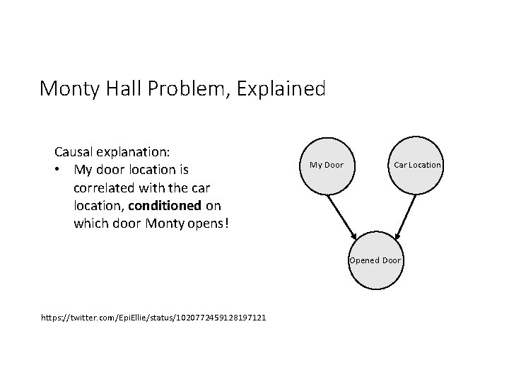
Monty Hall Problem, Explained Causal explanation: • My door location is correlated with the car location, conditioned on which door Monty opens! My Door Car Location Opened Door https: //twitter. com/Epi. Ellie/status/1020772459128197121

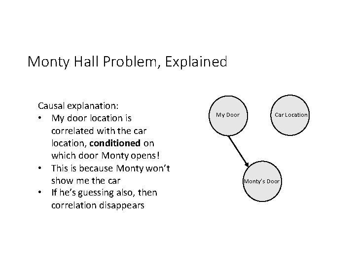
Monty Hall Problem, Explained Causal explanation: • My door location is correlated with the car location, conditioned on which door Monty opens! • This is because Monty won’t show me the car • If he’s guessing also, then correlation disappears My Door Car Location Monty’s Door

Structural Assumptions • All of this assumes that our assumptions about the DAG that generated our data are correct • Specifically, we assume that there are no hidden confounders • Confounder: a variable which causally effects both the treatment (T) and the outcome (Y) • No hidden confounders means that we have observed all confounders • This is a strong assumption!

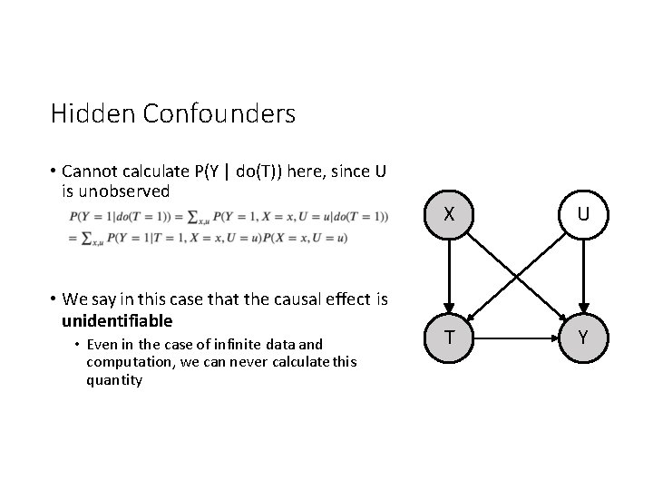
Hidden Confounders • Cannot calculate P(Y | do(T)) here, since U is unobserved • We say in this case that the causal effect is unidentifiable • Even in the case of infinite data and computation, we can never calculate this quantity X U T Y

What Can We Do with Hidden Confounders? • Instrumental variables • Find some variable which effects only the treatment • Sensitivity analysis • Essentially, assume some maximum amount of confounding • Yields confidence interval • Proxies • Other observed features give us information about the hidden confounder

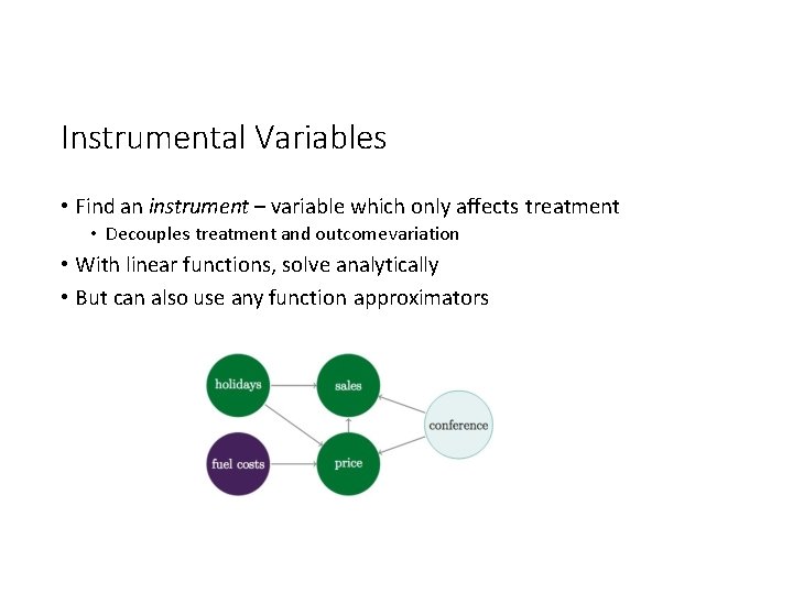
Instrumental Variables • Find an instrument – variable which only affects treatment • Decouples treatment and outcome variation • With linear functions, solve analytically • But can also use any function approximators

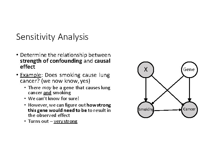
Sensitivity Analysis • Determine the relationship between strength of confounding and causal effect • Example: Does smoking cause lung cancer? (we now know, yes) • There may be a gene that causes lung cancer and smoking • We can’t know for sure! • However, we can figure out how strong this gene would need to be to result in the observed effect • Turns out – very strong X Gene Smoking Cancer

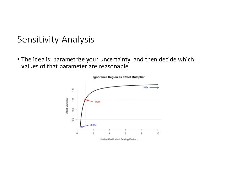
Sensitivity Analysis • The idea is: parametrize your uncertainty, and then decide which values of that parameter are reasonable

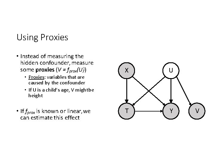
Using Proxies • Instead of measuring the hidden confounder, measure some proxies (V = fprox(U)) • Proxies: variables that are caused by the confounder • If U is a child’s age, V might be height • If fprox is known or linear, we can estimate this effect X U T Y V

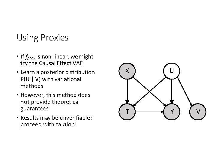
Using Proxies • If fprox is non-linear, we might try the Causal Effect VAE • Learn a posterior distribution P(U | V) with variational methods • However, this method does not provide theoretical guarantees • Results may be unverifiable: proceed with caution! X U T Y V

Causality and Other Areas of ML • Reinforcement Learning • Natural combination – RL is all about taking actions in the world • Off-policy learning already has elements of causal inference • Robust classification • Causality can be natural language for specifying distributional robustness • Fairness • If dataset is biased, ML outputs might be unfair • Causality helps us think about dataset bias, and mitigate unfair effects

Quick Note on Fairness and Causality • Many fairness problems (e. g. loans, medical diagnosis) are actually causal inference problems! • We talk about the label Y – however, this is not always observable • For instance, we can’t know if someone would return a loan if we don’t give one to them! • This means if we just train a classifier on historical data, our estimate will be biased • Biased in the fairness sense and the technical sense • General takeaway: if your data is generated by past decisions, think very hard about the output of your ML model!

Feedback Loops • Takes us to part 2… feedback loops • When ML systems are deployed, they make many decisions over time • So our past predictions can impact our future predictions! • Not good

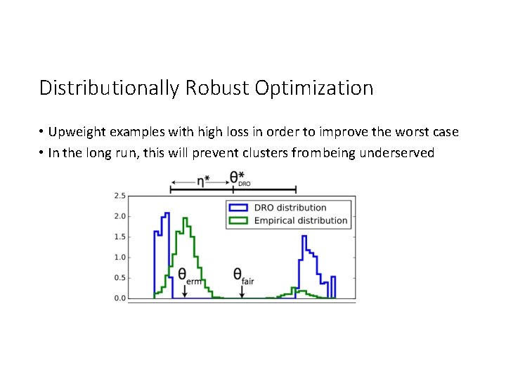
Unfair Feedback Loops • We’ll look at “Fairness Without Demographics in Repeated Loss Minimization” (Hashimoto et al, ICML 2018) • Domain: recommender systems • Suppose we have a majority group (A = 1) and minority group (A = 0) • Our recommender system may have high overall accuracy but low accuracy on the minority group • This can happen due to empirical risk minimization (ERM) • Can also be due to repeated decision-making

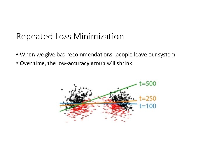
Repeated Loss Minimization • When we give bad recommendations, people leave our system • Over time, the low-accuracy group will shrink

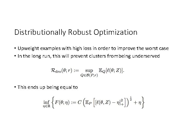
Distributionally Robust Optimization • Upweight examples with high loss in order to improve the worst case • In the long run, this will prevent clusters from being underserved • This ends up being equal to

Distributionally Robust Optimization • Upweight examples with high loss in order to improve the worst case • In the long run, this will prevent clusters from being underserved

Conclusion • Your data is not what it seems • ML models only work if your training/test set actually look like the environment you deploy them in • This can make your results unfair • Or just incorrect • So examine your model assumptions and data collection carefully!

The End

I will save money. • Choose 100 random people. • Watch which drugs they take and whether they are cured. Causal Inference Causal Graph D (Drug) X (Young/Old) Separate our people into these young/old. C (Cure) # people = 100 D (No Drug) D (Drug) # people = 50 (= 44 + 6) # people = 50 (= 10 +40) # Cured = 33 (= 31 + 2) # Cured = 25 (= 9 + 16) pr[ C | D ] = 25/50 = 0. 50 pr[ C | D ] = 33/50 = 0. 66 pr[C|D] - pr[C| D] = 0. 50 -0. 66 = -0. 16 Drug doesn't work X (Young) pr[ X] = (44+10)/100 = 0. 54 # people = 44 # Cured = 31 pr[ C | D & X ] = 31/44 = 0. 70 pr[ D | X] = 44/(44+10) = 0. 81 # people = 10 # Cured = 9 pr[ C | D & X ] = 9/10 = 0. 90 pr[ D | X ] = 10/(44+10) = 0. 19 X (Old) # people = 6 # Cured = 2 pr[ C | D & X] = 2/6 = 0. 33 pr[ D | X ] = 6/(6+40) = 0. 13 # people = 40 # Cured = 16 pr[ C | D & X ] = 16/40 = 0. 40 pr[ D | X ] = 40/(6+40) = 0. 87 pr[X] = (6+40)/100 = 0. 46