Chapter 7 Statistical Inference Statistical Inference Statistical inference

Chapter 7 Statistical Inference

Statistical Inference Statistical inference focuses on drawing conclusions about populations from samples. ◦ Statistical inference includes estimation of population parameters and hypothesis testing, which involves drawing conclusions about the value of the parameters of one or more populations.

Hypothesis Testing � Hypothesis testing involves drawing inferences about two contrasting propositions (each called a hypothesis) relating to the value of one or more population parameters. �H 0: Null hypothesis: describes an existing theory �H 1: Alternative hypothesis: the complement of H 0 � Using sample data, we either: - reject H 0 and conclude the sample data provides sufficient evidence to support H 1, or - fail to reject H 0 and conclude the sample data does not support H 1.

Example 7. 1: A Legal Analogy for Hypothesis Testing In the U. S. legal system, a defendant is innocent until proven guilty. ◦ H 0: Innocent ◦ H 1: Guilty If evidence (sample data) strongly indicates the defendant is guilty, then we reject H 0. Note that we have not proven guilt or innocence!

Hypothesis Testing Procedure Steps in conducting a hypothesis test: 1. Identify the population parameter and formulate the hypotheses to test. 2. Select a level of significance (the risk of drawing an incorrect conclusion). 3. Determine the decision rule on which to base a conclusion. 4. Collect data and calculate a test statistic. 5. Apply the decision rule and draw a conclusion.

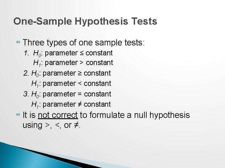
One-Sample Hypothesis Tests Three types of one sample tests: 1. H 0: parameter ≤ constant H 1: parameter > constant 2. H 0: parameter ≥ constant H 1: parameter < constant 3. H 0: parameter = constant H 1: parameter ≠ constant It is not correct to formulate a null hypothesis using >, <, or ≠.

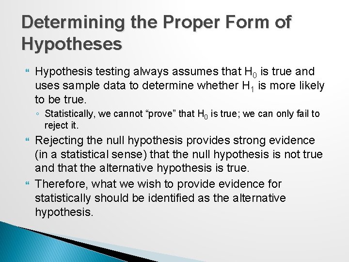
Determining the Proper Form of Hypotheses Hypothesis testing always assumes that H 0 is true and uses sample data to determine whether H 1 is more likely to be true. ◦ Statistically, we cannot “prove” that H 0 is true; we can only fail to reject it. Rejecting the null hypothesis provides strong evidence (in a statistical sense) that the null hypothesis is not true and that the alternative hypothesis is true. Therefore, what we wish to provide evidence for statistically should be identified as the alternative hypothesis.

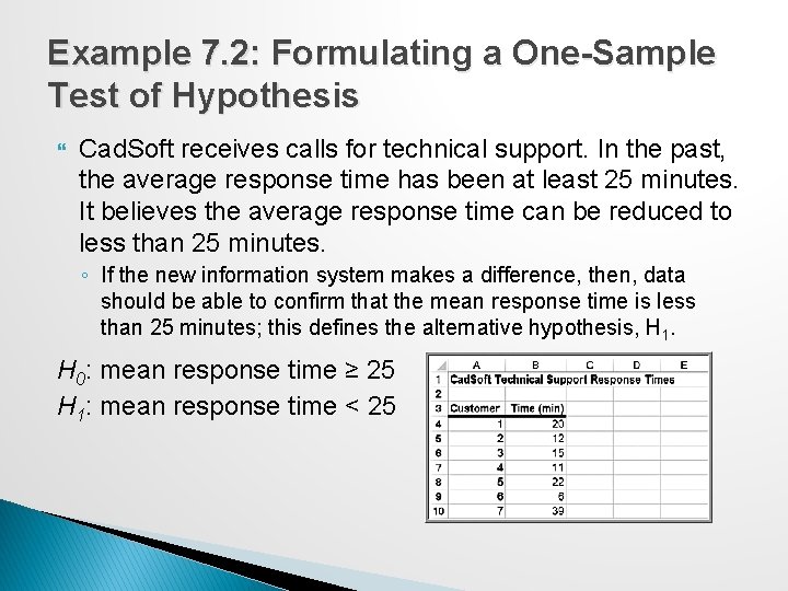
Example 7. 2: Formulating a One-Sample Test of Hypothesis Cad. Soft receives calls for technical support. In the past, the average response time has been at least 25 minutes. It believes the average response time can be reduced to less than 25 minutes. ◦ If the new information system makes a difference, then, data should be able to confirm that the mean response time is less than 25 minutes; this defines the alternative hypothesis, H 1. H 0: mean response time ≥ 25 H 1: mean response time < 25

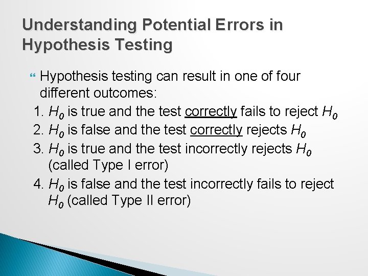
Understanding Potential Errors in Hypothesis Testing Hypothesis testing can result in one of four different outcomes: 1. H 0 is true and the test correctly fails to reject H 0 2. H 0 is false and the test correctly rejects H 0 3. H 0 is true and the test incorrectly rejects H 0 (called Type I error) 4. H 0 is false and the test incorrectly fails to reject H 0 (called Type II error)

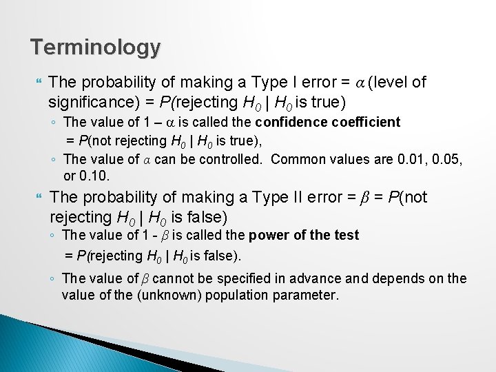
Terminology The probability of making a Type I error = α (level of significance) = P(rejecting H 0 | H 0 is true) ◦ The value of 1 – a is called the confidence coefficient = P(not rejecting H 0 | H 0 is true), ◦ The value of α can be controlled. Common values are 0. 01, 0. 05, or 0. 10. The probability of making a Type II error = β = P(not rejecting H 0 | H 0 is false) ◦ The value of 1 - β is called the power of the test = P(rejecting H 0 | H 0 is false). ◦ The value of β cannot be specified in advance and depends on the value of the (unknown) population parameter.

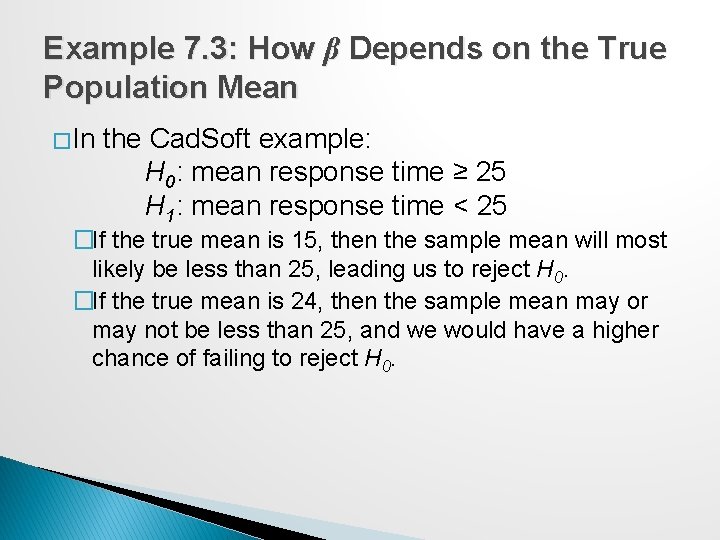
Example 7. 3: How β Depends on the True Population Mean � In the Cad. Soft example: H 0: mean response time ≥ 25 H 1: mean response time < 25 �If the true mean is 15, then the sample mean will most likely be less than 25, leading us to reject H 0. �If the true mean is 24, then the sample mean may or may not be less than 25, and we would have a higher chance of failing to reject H 0.

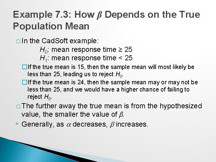
Example 7. 3: How β Depends on the True Population Mean � In the Cad. Soft example: H 0: mean response time ≥ 25 H 1: mean response time < 25 �If the true mean is 15, then the sample mean will most likely be less than 25, leading us to reject H 0. �If the true mean is 24, then the sample mean may or may not be less than 25, and we would have a higher chance of failing to reject H 0. � The further away the true mean is from the hypothesized value, the smaller the value of β. Generally, as a decreases, b increases.

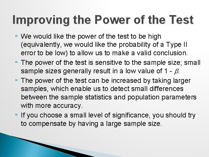
Improving the Power of the Test We would like the power of the test to be high (equivalently, we would like the probability of a Type II error to be low) to allow us to make a valid conclusion. The power of the test is sensitive to the sample size; small sample sizes generally result in a low value of 1 - b. The power of the test can be increased by taking larger samples, which enable us to detect small differences between the sample statistics and population parameters with more accuracy. If you choose a small level of significance, you should try to compensate by having a large sample size.

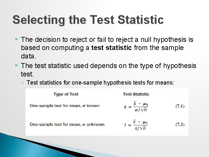
Selecting the Test Statistic The decision to reject or fail to reject a null hypothesis is based on computing a test statistic from the sample data. The test statistic used depends on the type of hypothesis test. ◦ Test statistics for one-sample hypothesis tests for means:

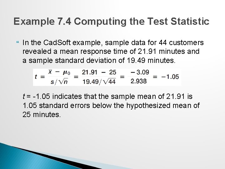
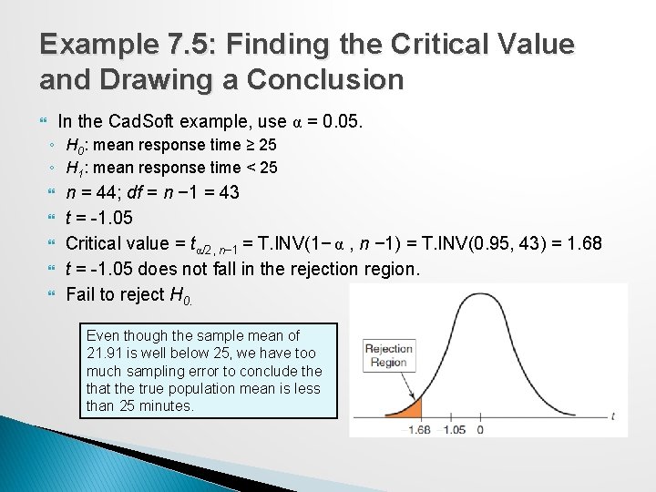
Example 7. 4 Computing the Test Statistic In the Cad. Soft example, sample data for 44 customers revealed a mean response time of 21. 91 minutes and a sample standard deviation of 19. 49 minutes. t = -1. 05 indicates that the sample mean of 21. 91 is 1. 05 standard errors below the hypothesized mean of 25 minutes.

Drawing a Conclusion The conclusion to reject or fail to reject H 0 is based on comparing the value of the test statistic to a “critical value” from the sampling distribution of the test statistic when the null hypothesis is true and the chosen level of significance, a. ◦ The sampling distribution of the test statistic is usually the normal distribution, t-distribution, or some other well-known distribution. The critical value divides the sampling distribution into two parts, a rejection region and a non-rejection region. If the test statistic falls into the rejection region, we reject the null hypothesis; otherwise, we fail to reject it.

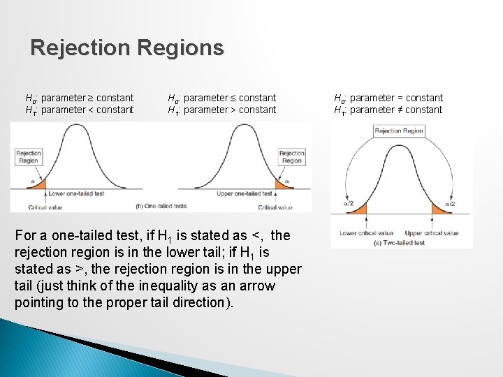
Rejection Regions H 0: parameter ≥ constant H 1: parameter < constant H 0: parameter ≤ constant H 1: parameter > constant For a one-tailed test, if H 1 is stated as <, the rejection region is in the lower tail; if H 1 is stated as >, the rejection region is in the upper tail (just think of the inequality as an arrow pointing to the proper tail direction). H 0: parameter = constant H 1: parameter ≠ constant

Example 7. 5: Finding the Critical Value and Drawing a Conclusion In the Cad. Soft example, use α = 0. 05. ◦ H 0: mean response time ≥ 25 ◦ H 1: mean response time < 25 n = 44; df = n − 1 = 43 t = -1. 05 Critical value = tα/2, n− 1 = T. INV(1− α , n − 1) = T. INV(0. 95, 43) = 1. 68 t = -1. 05 does not fall in the rejection region. Fail to reject H 0. Even though the sample mean of 21. 91 is well below 25, we have too much sampling error to conclude that the true population mean is less than 25 minutes.

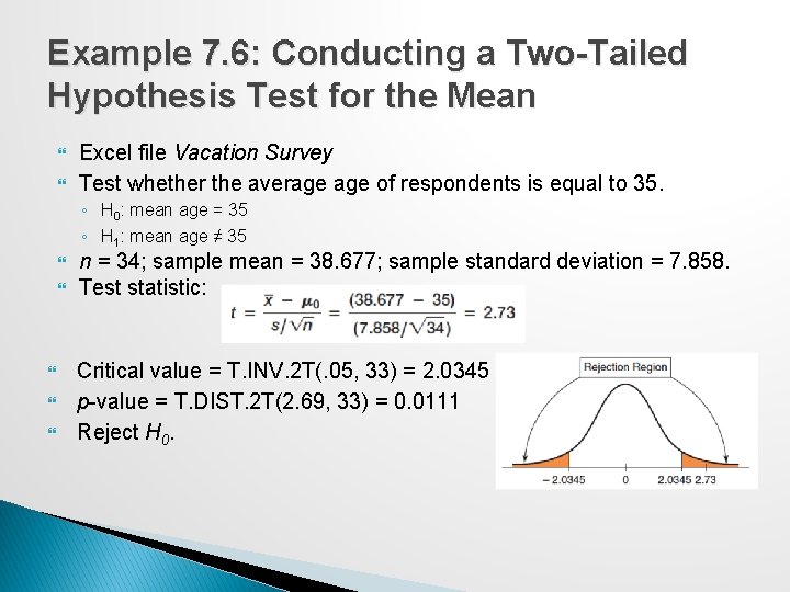
Example 7. 6: Conducting a Two-Tailed Hypothesis Test for the Mean Excel file Vacation Survey Test whether the average of respondents is equal to 35. ◦ H 0: mean age = 35 ◦ H 1: mean age ≠ 35 n = 34; sample mean = 38. 677; sample standard deviation = 7. 858. Test statistic: Critical value = T. INV. 2 T(. 05, 33) = 2. 0345 p-value = T. DIST. 2 T(2. 69, 33) = 0. 0111 Reject H 0.

p-Values A p-value (observed significance level) is the probability of obtaining a test statistic value equal to or more extreme than that obtained from the sample data when the null hypothesis is true. � An alternative approach to Step 3 of a hypothesis test uses the p-value rather than the critical value: Reject H 0 if the p-value < α

Finding p-Values For a lower one-tailed test, the p-value is the probability to the left of the test statistic t in the t-distribution, and is found using the Excel function: ◦ =T. DIST(t, n-1, TRUE). For an upper one-tailed test, the p-value is the probability to the right of the test statistic t, and is found using the Excel function: ◦ 1 - T. DIST(t, n-1, TRUE). For a two-tailed test, the p-value is found using the Excel function: ◦ T. DIST. 2 T(t, n-1), if t > 0 ◦ T. DIST. 2 T(-t, n-1), if t < 0

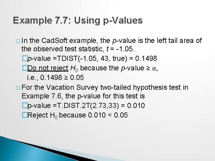
Example 7. 7: Using p-Values � In the Cad. Soft example, the p-value is the left tail area of the observed test statistic, t = -1. 05. �p-value =TDIST(-1. 05, 43, true) = 0. 1498 �Do not reject H 0 because the p-value ≥ α, i. e. , 0. 1498 ≥ 0. 05 � For the Vacation Survey two-tailed hypothesis test in Example 7. 6, the p-value for this test is �p-value =T. DIST. 2 T(2. 73, 33) = 0. 010 �Reject H 0 because 0. 010 < 0. 05

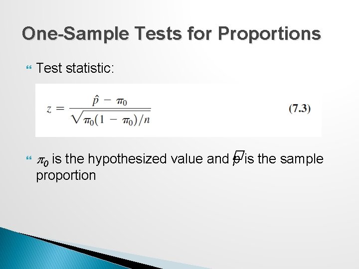
One-Sample Tests for Proportions Test statistic: p 0 is the hypothesized value and � p is the sample proportion

Example 7. 8: One-Sample Test for the Proportion Cad. Soft sampled 44 customers and asked them to rate the overall quality of a software package. Sample data revealed that 35 respondents (a proportion of 35/44 = 0. 795) thought the software was very good or excellent. In the past, this proportion has averaged about 75%. Is there sufficient evidence to conclude that this satisfaction measure has significantly exceeded 75% using a significance level of 0. 05?

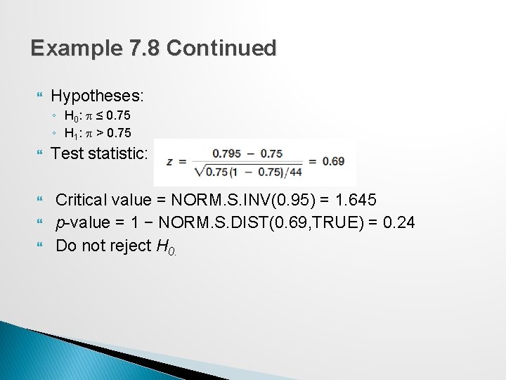
Example 7. 8 Continued Hypotheses: ◦ H 0: p ≤ 0. 75 ◦ H 1: p > 0. 75 Test statistic: Critical value = NORM. S. INV(0. 95) = 1. 645 p-value = 1 − NORM. S. DIST(0. 69, TRUE) = 0. 24 Do not reject H 0.

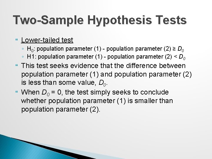
Two-Sample Hypothesis Tests Lower-tailed test ◦ H 0: population parameter (1) - population parameter (2) ≥ D 0 ◦ H 1: population parameter (1) - population parameter (2) < D 0 This test seeks evidence that the difference between population parameter (1) and population parameter (2) is less than some value, D 0. When D 0 = 0, the test simply seeks to conclude whether population parameter (1) is smaller than population parameter (2).

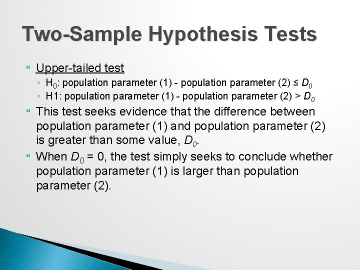
Two-Sample Hypothesis Tests Upper-tailed test ◦ H 0: population parameter (1) - population parameter (2) ≤ D 0 ◦ H 1: population parameter (1) - population parameter (2) > D 0 This test seeks evidence that the difference between population parameter (1) and population parameter (2) is greater than some value, D 0. When D 0 = 0, the test simply seeks to conclude whether population parameter (1) is larger than population parameter (2).

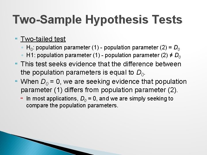
Two-Sample Hypothesis Tests Two-tailed test ◦ H 0: population parameter (1) - population parameter (2) = D 0 ◦ H 1: population parameter (1) - population parameter (2) ≠ D 0 This test seeks evidence that the difference between the population parameters is equal to D 0. When D 0 = 0, we are seeking evidence that population parameter (1) differs from population parameter (2). In most applications, D 0 = 0, and we are simply seeking to compare the population parameters.

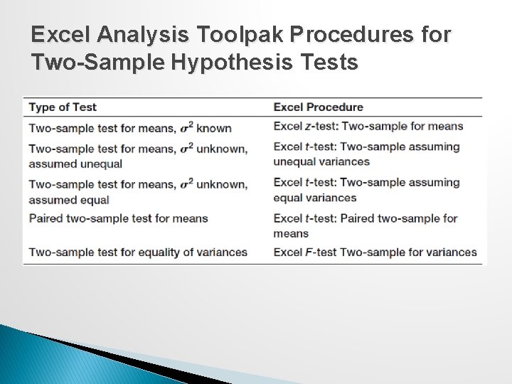
Excel Analysis Toolpak Procedures for Two-Sample Hypothesis Tests

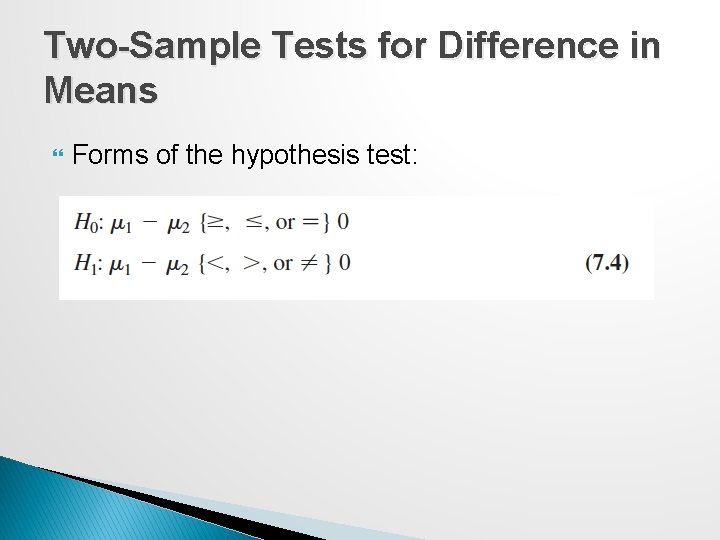
Two-Sample Tests for Difference in Means Forms of the hypothesis test:

Example 7. 9: Comparing Supplier Performance Purchase Orders database Determine if the mean lead time for Alum Sheeting (µ 1) is greater than the mean lead time for Durrable Products (µ 2).

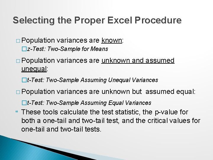
Selecting the Proper Excel Procedure � Population variances are known: �z-Test: Two-Sample for Means � Population variances are unknown and assumed unequal: �t-Test: Two-Sample Assuming Unequal Variances � Population variances are unknown but assumed equal: �t-Test: Two-Sample Assuming Equal Variances These tools calculate the test statistic, the p-value for both a one-tail and two-tail test, and the critical values for one-tail and two-tail tests.

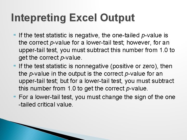
Intepreting Excel Output If the test statistic is negative, the one-tailed p-value is the correct p-value for a lower-tail test; however, for an upper-tail test, you must subtract this number from 1. 0 to get the correct p-value. If the test statistic is nonnegative (positive or zero), then the p-value in the output is the correct p-value for an upper-tail test; but for a lower-tail test, you must subtract this number from 1. 0 to get the correct p-value. For a lower-tail test, you must change the sign of the one -tailed critical value.

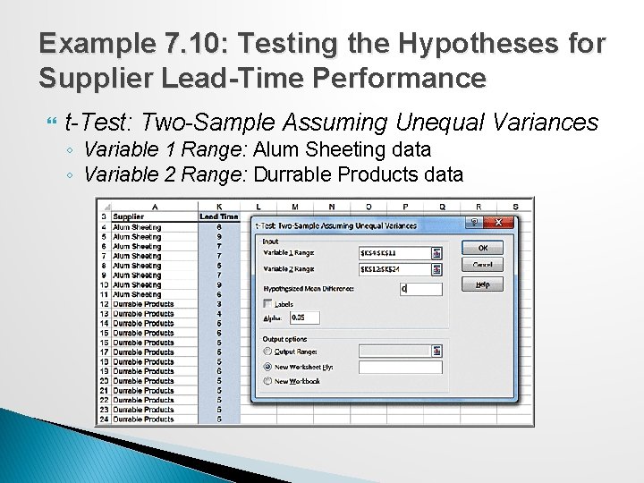
Example 7. 10: Testing the Hypotheses for Supplier Lead-Time Performance t-Test: Two-Sample Assuming Unequal Variances ◦ Variable 1 Range: Alum Sheeting data ◦ Variable 2 Range: Durrable Products data

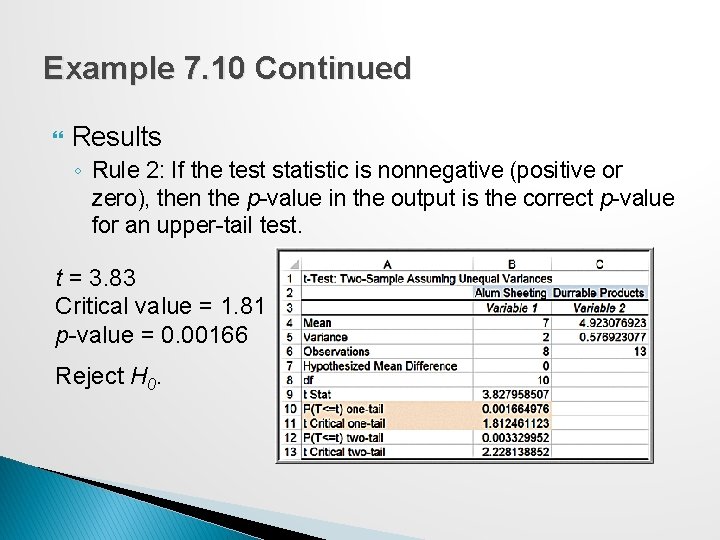
Example 7. 10 Continued Results ◦ Rule 2: If the test statistic is nonnegative (positive or zero), then the p-value in the output is the correct p-value for an upper-tail test. t = 3. 83 Critical value = 1. 81 p-value = 0. 00166 Reject H 0.

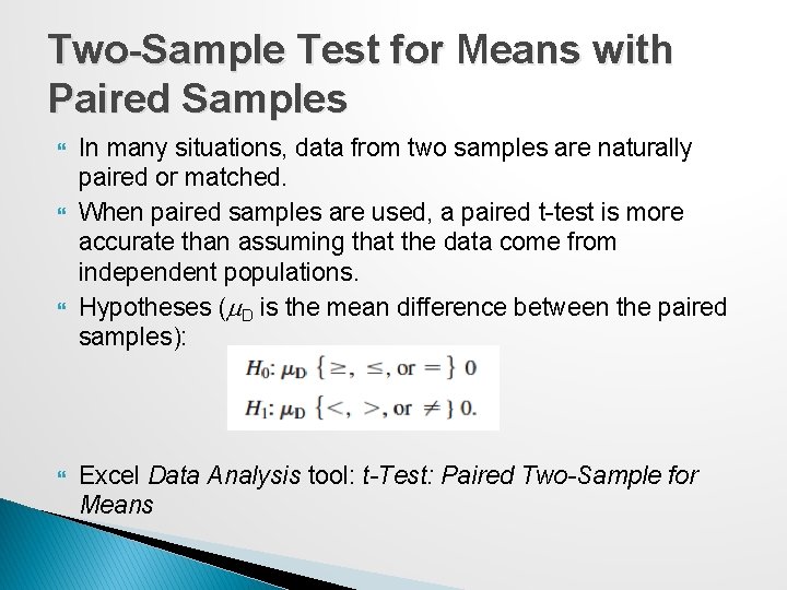
Two-Sample Test for Means with Paired Samples In many situations, data from two samples are naturally paired or matched. When paired samples are used, a paired t-test is more accurate than assuming that the data come from independent populations. Hypotheses (m. D is the mean difference between the paired samples): Excel Data Analysis tool: t-Test: Paired Two-Sample for Means

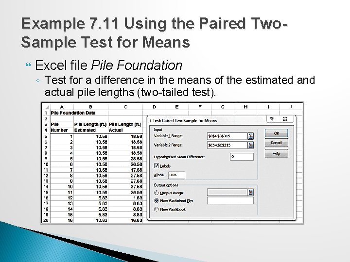
Example 7. 11 Using the Paired Two. Sample Test for Means Excel file Pile Foundation ◦ Test for a difference in the means of the estimated and actual pile lengths (two-tailed test).

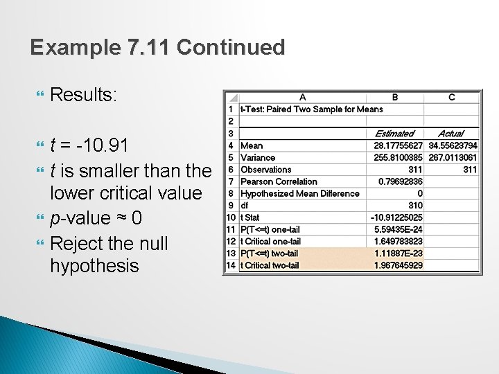
Example 7. 11 Continued Results: t = -10. 91 t is smaller than the lower critical value p-value ≈ 0 Reject the null hypothesis

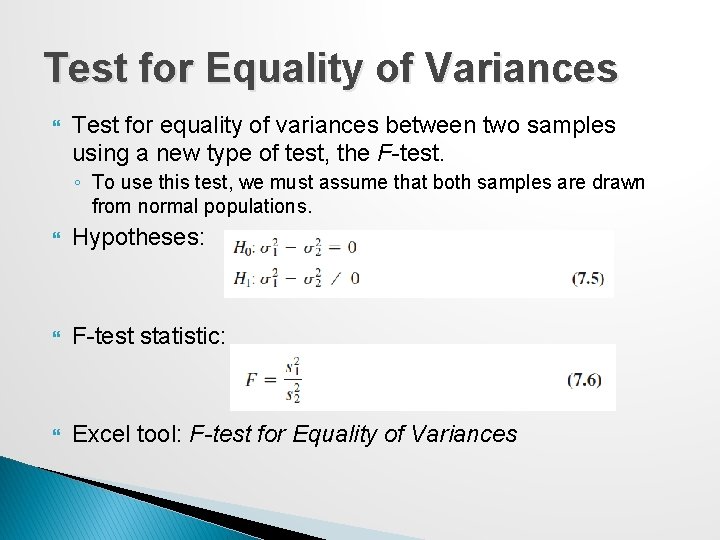
Test for Equality of Variances Test for equality of variances between two samples using a new type of test, the F-test. ◦ To use this test, we must assume that both samples are drawn from normal populations. Hypotheses: F-test statistic: Excel tool: F-test for Equality of Variances

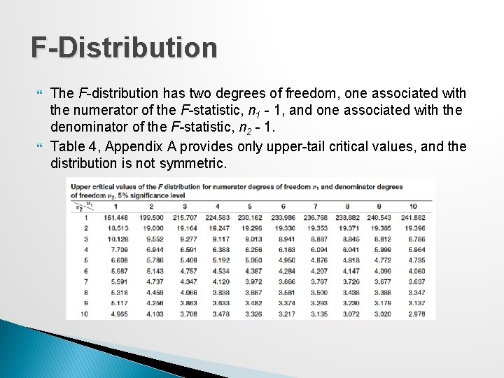
F-Distribution The F-distribution has two degrees of freedom, one associated with the numerator of the F-statistic, n 1 - 1, and one associated with the denominator of the F-statistic, n 2 - 1. Table 4, Appendix A provides only upper-tail critical values, and the distribution is not symmetric.

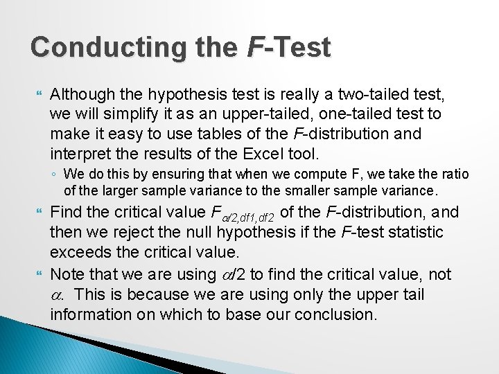
Conducting the F-Test Although the hypothesis test is really a two-tailed test, we will simplify it as an upper-tailed, one-tailed test to make it easy to use tables of the F-distribution and interpret the results of the Excel tool. ◦ We do this by ensuring that when we compute F, we take the ratio of the larger sample variance to the smaller sample variance. Find the critical value Fa/2, df 1, df 2 of the F-distribution, and then we reject the null hypothesis if the F-test statistic exceeds the critical value. Note that we are using a/2 to find the critical value, not a. This is because we are using only the upper tail information on which to base our conclusion.

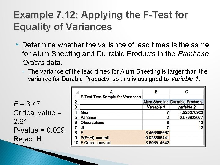
Example 7. 12: Applying the F-Test for Equality of Variances Determine whether the variance of lead times is the same for Alum Sheeting and Durrable Products in the Purchase Orders data. ◦ The variance of the lead times for Alum Sheeting is larger than the variance for Durable Products, so this is assigned to Variable 1. F = 3. 47 Critical value = 2. 91 P-value = 0. 029 Reject H 0

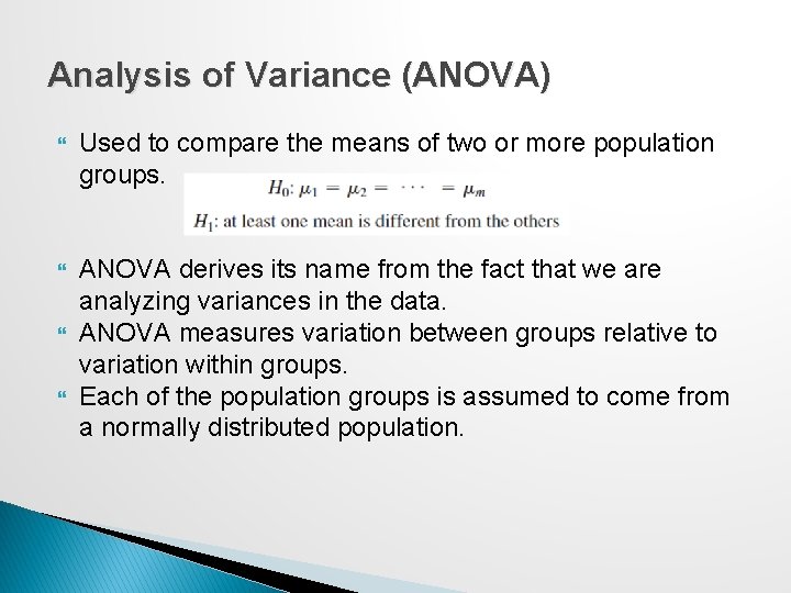
Analysis of Variance (ANOVA) Used to compare the means of two or more population groups. ANOVA derives its name from the fact that we are analyzing variances in the data. ANOVA measures variation between groups relative to variation within groups. Each of the population groups is assumed to come from a normally distributed population.

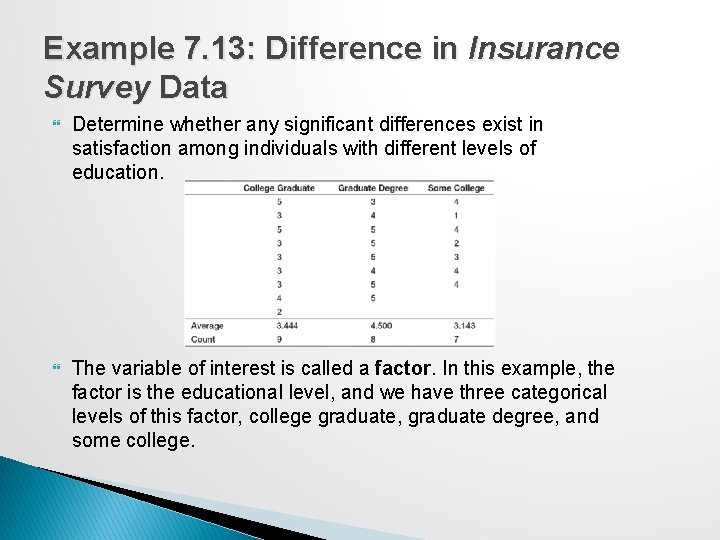
Example 7. 13: Difference in Insurance Survey Data Determine whether any significant differences exist in satisfaction among individuals with different levels of education. The variable of interest is called a factor. In this example, the factor is the educational level, and we have three categorical levels of this factor, college graduate, graduate degree, and some college.

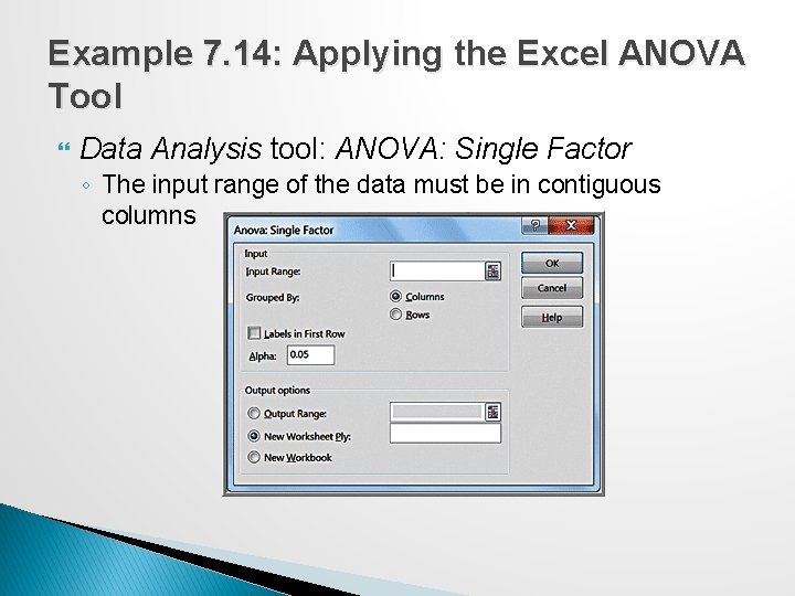
Example 7. 14: Applying the Excel ANOVA Tool Data Analysis tool: ANOVA: Single Factor ◦ The input range of the data must be in contiguous columns

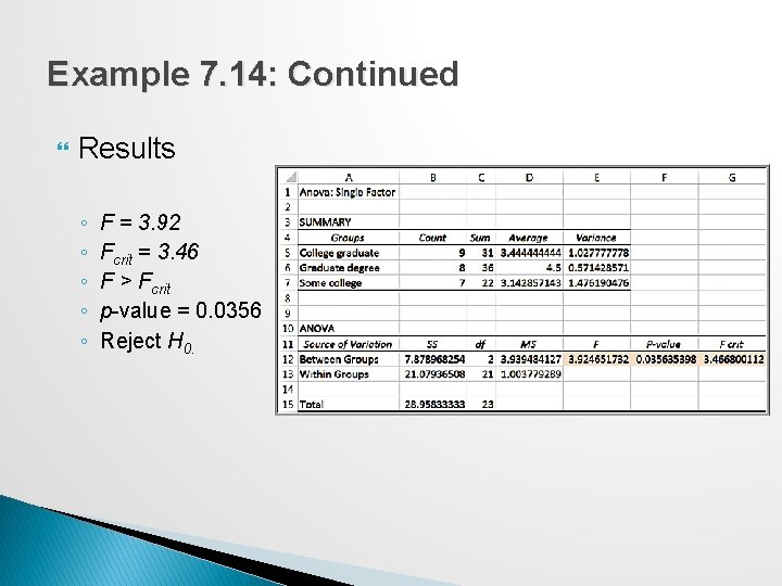
Example 7. 14: Continued Results ◦ ◦ ◦ F = 3. 92 Fcrit = 3. 46 F > Fcrit p-value = 0. 0356 Reject H 0.

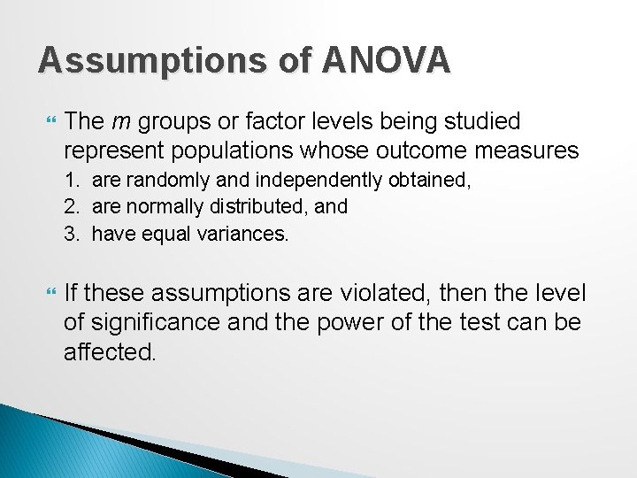
Assumptions of ANOVA The m groups or factor levels being studied represent populations whose outcome measures 1. are randomly and independently obtained, 2. are normally distributed, and 3. have equal variances. If these assumptions are violated, then the level of significance and the power of the test can be affected.

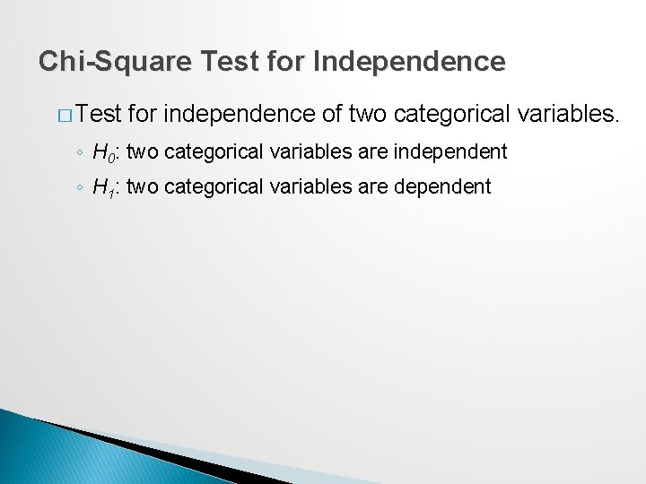
Chi-Square Test for Independence � Test for independence of two categorical variables. ◦ H 0: two categorical variables are independent ◦ H 1: two categorical variables are dependent

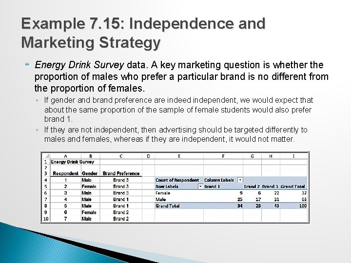
Example 7. 15: Independence and Marketing Strategy Energy Drink Survey data. A key marketing question is whether the proportion of males who prefer a particular brand is no different from the proportion of females. ◦ If gender and brand preference are indeed independent, we would expect that about the same proportion of the sample of female students would also prefer brand 1. ◦ If they are not independent, then advertising should be targeted differently to males and females, whereas if they are independent, it would not matter.

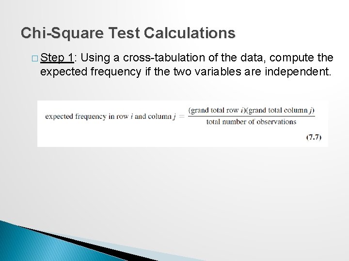
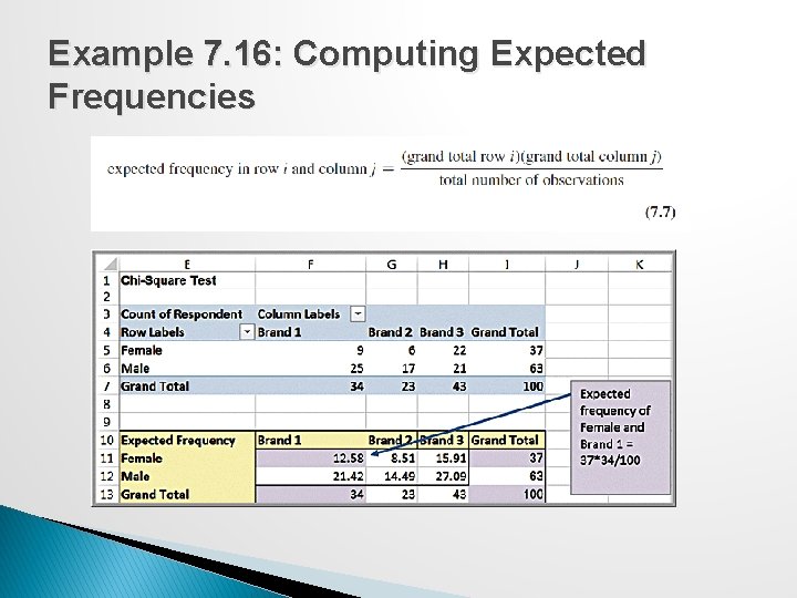
Chi-Square Test Calculations � Step 1: Using a cross-tabulation of the data, compute the expected frequency if the two variables are independent.

Example 7. 16: Computing Expected Frequencies

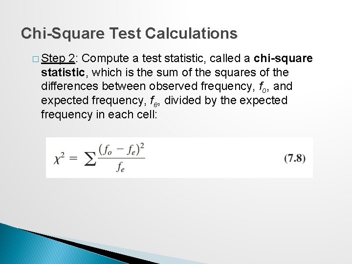
Chi-Square Test Calculations � Step 2: Compute a test statistic, called a chi-square statistic, which is the sum of the squares of the differences between observed frequency, fo, and expected frequency, fe, divided by the expected frequency in each cell:

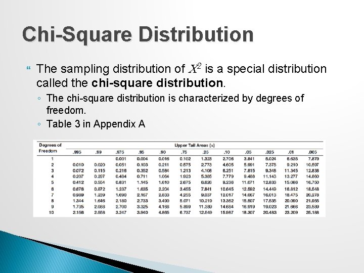
Chi-Square Distribution The sampling distribution of C 2 is a special distribution called the chi-square distribution. ◦ The chi-square distribution is characterized by degrees of freedom. ◦ Table 3 in Appendix A

Chi-Square Test Calculations (continued) Step 3: Compare the chi-square statistic for the level of significance a to the critical value from a chi-square distribution with (r – 1)(c – 1) degrees of freedom, where r and c are the number of rows and columns in the cross-tabulation table, respectively. ◦ The Excel function CHISQ. INV. RT(probability, deg_ freedom) returns the value of C 2 that has a right-tail area equal to probability for a specified degree of freedom. ◦ By setting probability equal to the level of significance, we can obtain the critical value for the hypothesis test. ◦ The Excel function CHISQ. TEST(actual_range, expected_range) computes the p-value for the chi-square test.

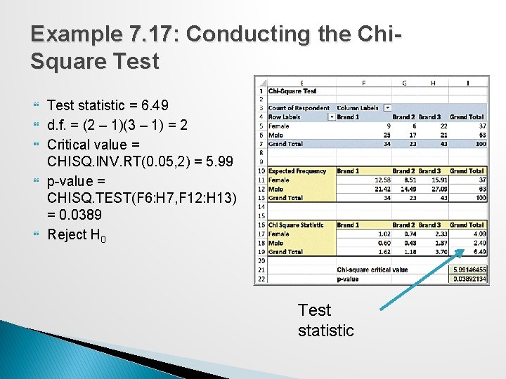
Example 7. 17: Conducting the Chi. Square Test statistic = 6. 49 d. f. = (2 – 1)(3 – 1) = 2 Critical value = CHISQ. INV. RT(0. 05, 2) = 5. 99 p-value = CHISQ. TEST(F 6: H 7, F 12: H 13) = 0. 0389 Reject H 0 Test statistic