Statistical inference Statistical inference n Definition generalization from

Statistical inference

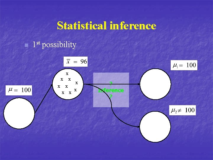
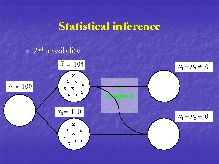
Statistical inference n Definition : generalization from a sample to a population. n 2 cases: n n Is a sample belongs to an hypothetical population? Is two samples belong to the same hypothetical population?

Statistical inference n 1 st possibility x x x x x ? Inference ?

Statistical inference n 2 nd possibility x x x x x ? Inference ?

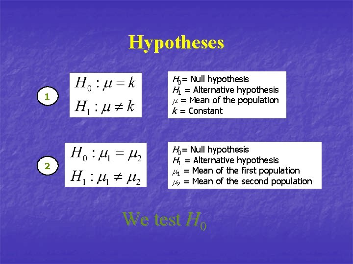
Hypotheses 1 H 0= Null hypothesis H 1 = Alternative hypothesis m = Mean of the population k = Constant 2 H 0= Null hypothesis H 1 = Alternative hypothesis m 1 = Mean of the first population m 2 = Mean of the second population We test H 0

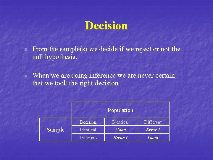
Decision n From the sample(s) we decide if we reject or not the null hypothesis. n When we are doing inference we are never certain that we took the right decision Population Sample Decision Identical Different Identical Good Error 2 Different Error 1 Good

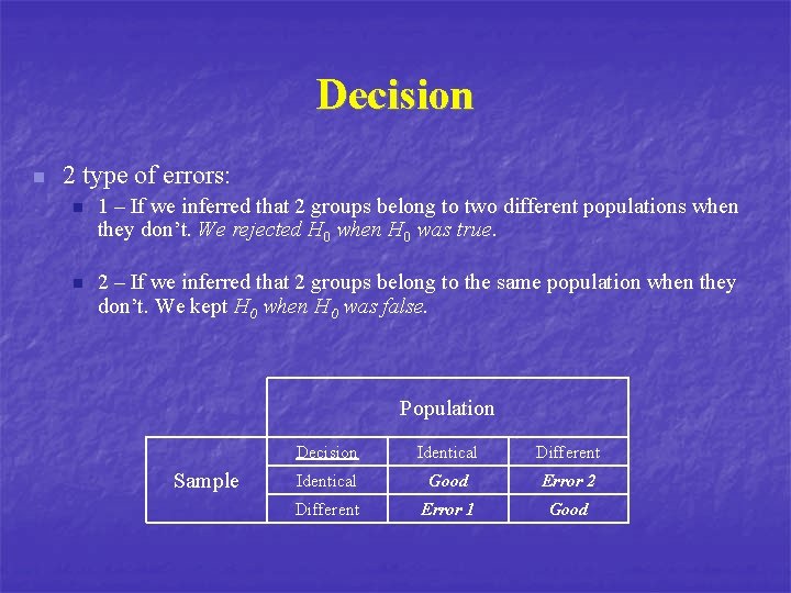
Decision n 2 type of errors: n 1 – If we inferred that 2 groups belong to two different populations when they don’t. We rejected H 0 when H 0 was true. n 2 – If we inferred that 2 groups belong to the same population when they don’t. We kept H 0 when H 0 was false. Population Sample Decision Identical Different Identical Good Error 2 Different Error 1 Good

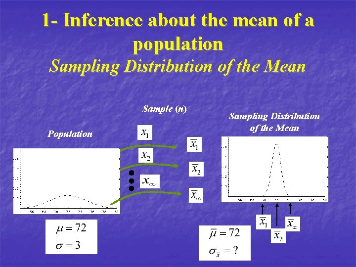
1 - Inference about the mean of a population Sampling Distribution of the Mean Sample (n) Population Sampling Distribution of the Mean

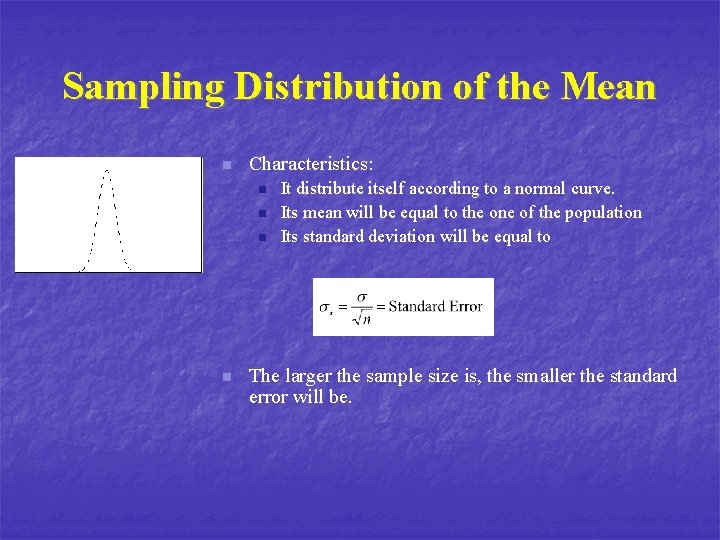
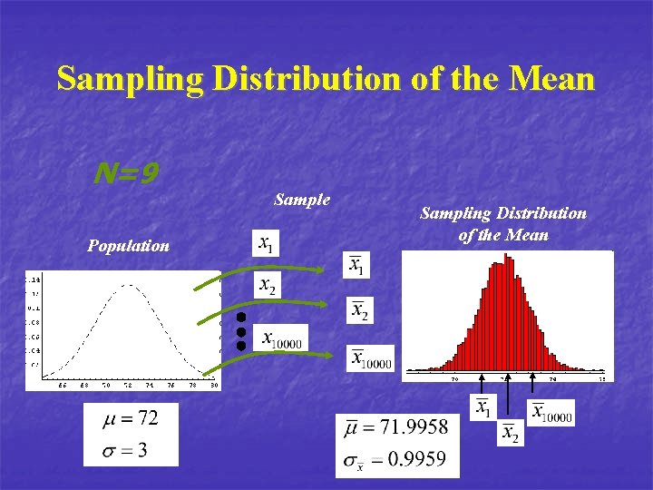
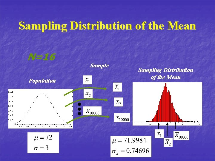
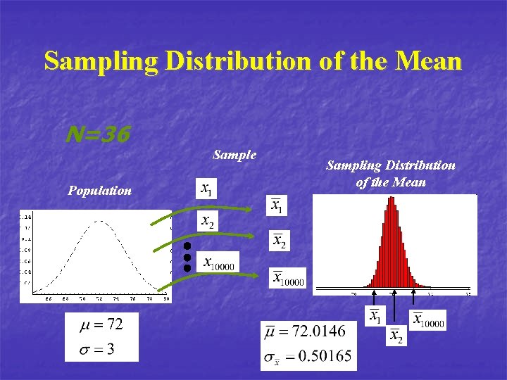
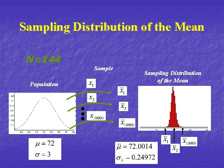
Sampling Distribution of the Mean n Characteristics: n n It distribute itself according to a normal curve. Its mean will be equal to the one of the population Its standard deviation will be equal to The larger the sample size is, the smaller the standard error will be.

Sampling Distribution of the Mean N=9 Population Sample Sampling Distribution of the Mean

Sampling Distribution of the Mean N=16 Population Sample Sampling Distribution of the Mean

Sampling Distribution of the Mean N=36 Population Sample Sampling Distribution of the Mean

Sampling Distribution of the Mean N=144 Population Sample Sampling Distribution of the Mean

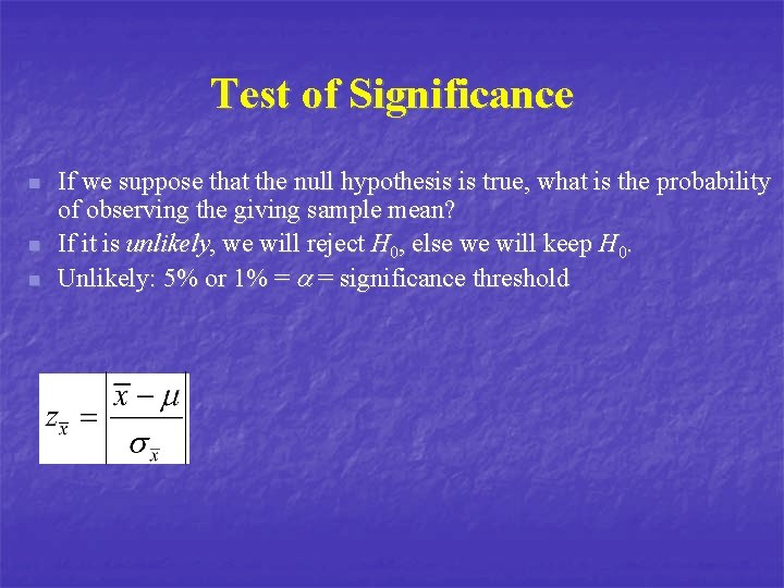
Test of Significance n n n If we suppose that the null hypothesis is true, what is the probability of observing the giving sample mean? If it is unlikely, we will reject H 0, else we will keep H 0. Unlikely: 5% or 1% = a = significance threshold

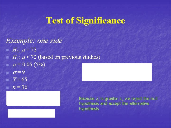
Test of Significance Example: one side n n n H 0: m = 72 H 1: m < 72 (based on previous studies) a = 0. 05 (5%) s=9 = 65 n = 36 Because zx is greater za we reject the null hypothesis and accept the alternative hypothesis za = 1. 65

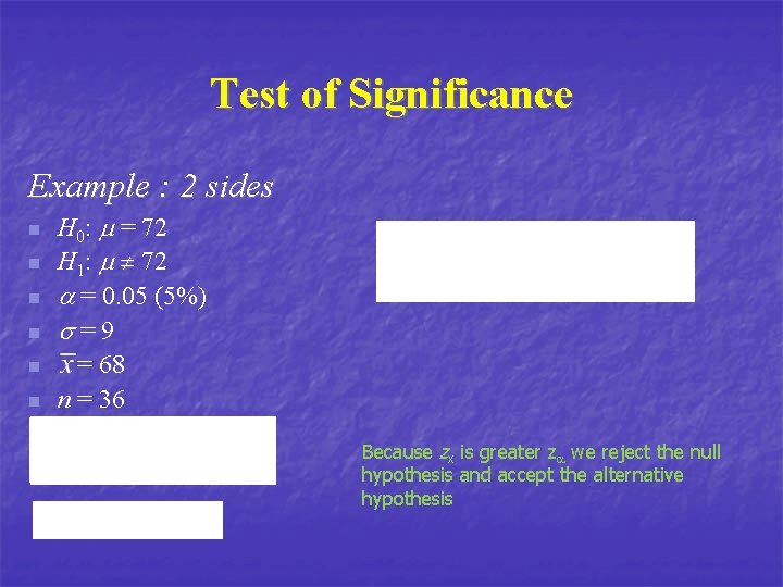
Test of Significance Example : 2 sides n n n H 0: m = 72 H 1: m 72 a = 0. 05 (5%) s=9 = 68 n = 36 Because zx is greater za we reject the null hypothesis and accept the alternative hypothesis za = 1. 96

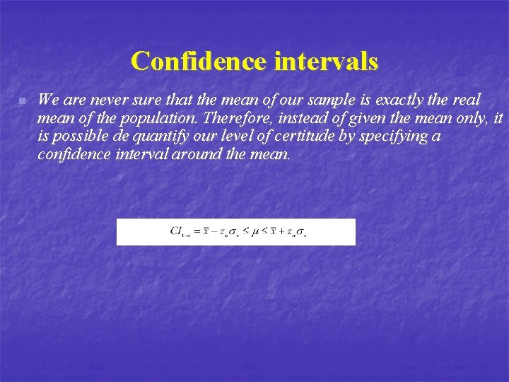
Confidence intervals n We are never sure that the mean of our sample is exactly the real mean of the population. Therefore, instead of given the mean only, it is possible de quantify our level of certitude by specifying a confidence interval around the mean.

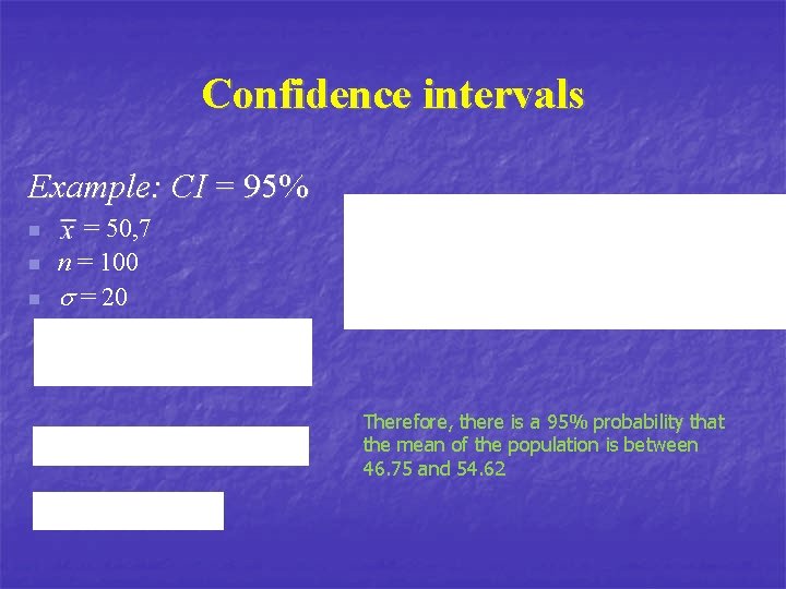
Confidence intervals Example: CI = 95% n n n = 50, 7 n = 100 s = 20 Therefore, there is a 95% probability that the mean of the population is between 46. 75 and 54. 62 za = 1. 96

Confidence intervals Example: CI = 99% n n n = 50, 7 n = 100 s = 20 Therefore, there is a 99% probability that the mean of the population is between 445. 54 and 55. 86 za = 1. 96