CS 188 Artificial Intelligence Bayes Nets Inference Instructors

CS 188: Artificial Intelligence Bayes’ Nets: Inference Instructors: Anca Dragan --- University of California, Berkeley [Slides by Dan Klein, Pieter Abbeel, Anca Dragan. http: //ai. berkeley. edu. ]
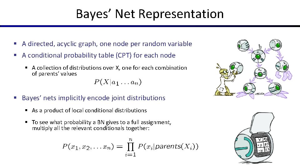
Bayes’ Net Representation § A directed, acyclic graph, one node per random variable § A conditional probability table (CPT) for each node § A collection of distributions over X, one for each combination of parents’ values § Bayes’ nets implicitly encode joint distributions § As a product of local conditional distributions § To see what probability a BN gives to a full assignment, multiply all the relevant conditionals together:

Example: Alarm Network B P(B) +b 0. 001 -b 0. 999 Burglary Earthqk E P(E) +e 0. 002 -e 0. 998 Alarm John calls Mary calls B E A P(A|B, E) +b +e +a 0. 95 +b +e -a 0. 05 +b -e +a 0. 94 A J P(J|A) A M P(M|A) +b -e -a 0. 06 +a +j 0. 9 +a +m 0. 7 -b +e +a 0. 29 +a -j 0. 1 +a -m 0. 3 -b +e -a 0. 71 -a +j 0. 05 -a +m 0. 01 -b -e +a 0. 001 -a -j 0. 95 -a -m 0. 99 -b -e -a 0. 999
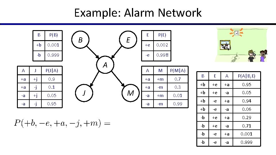
Example: Alarm Network B P(B) +b 0. 001 -b 0. 999 A J P(J|A) +a +j +a B E A E P(E) +e 0. 002 -e 0. 998 A M P(M|A) 0. 9 +a +m 0. 7 -j 0. 1 +a -m 0. 3 -a +j 0. 05 -a +m 0. 01 -a -j 0. 95 -a -m 0. 99 J M B E A P(A|B, E) +b +e +a 0. 95 +b +e -a 0. 05 +b -e +a 0. 94 +b -e -a 0. 06 -b +e +a 0. 29 -b +e -a 0. 71 -b -e +a 0. 001 -b -e -a 0. 999
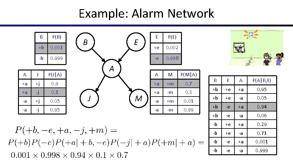
Example: Alarm Network B P(B) +b 0. 001 -b 0. 999 A J P(J|A) +a +j +a B E A E P(E) +e 0. 002 -e 0. 998 A M P(M|A) 0. 9 +a +m 0. 7 -j 0. 1 +a -m 0. 3 -a +j 0. 05 -a +m 0. 01 -a -j 0. 95 -a -m 0. 99 J M B E A P(A|B, E) +b +e +a 0. 95 +b +e -a 0. 05 +b -e +a 0. 94 +b -e -a 0. 06 -b +e +a 0. 29 -b +e -a 0. 71 -b -e +a 0. 001 -b -e -a 0. 999

Inference § Inference: calculating some useful quantity from a joint probability distribution § Examples: § Posterior probability § Most likely explanation:
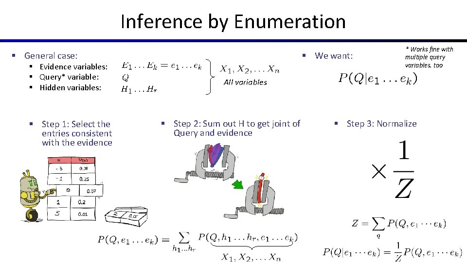
Inference by Enumeration § General case: § Evidence variables: § Query* variable: § Hidden variables: § Step 1: Select the entries consistent with the evidence § We want: * Works fine with multiple query variables, too All variables § Step 2: Sum out H to get joint of Query and evidence § Step 3: Normalize
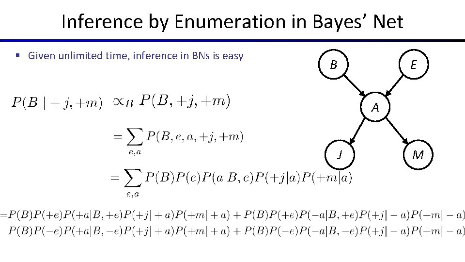
Inference by Enumeration in Bayes’ Net § Given unlimited time, inference in BNs is easy B E A J M

Inference by Enumeration § General case: § We want: § Evidence variables: § Query* variable: § Hidden variables: § Step 1: Select the entries consistent with the evidence * Works fine with multiple query variables, too All variables § Step 2: Sum out H to get joint of Query and evidence § Compute joint § Sum out hidden variables § Step 3: Normalize

Example: Traffic Domain § Random Variables § R: Raining § T: Traffic § L: Late for class! +r -r R T L 0. 1 0. 9 +r +r -r -r +t -t 0. 8 0. 2 0. 1 0. 9 +t +t -t -t +l -l 0. 3 0. 7 0. 1 0. 9
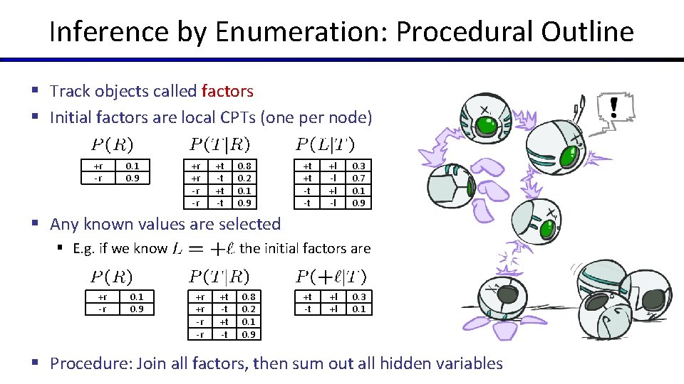
Inference by Enumeration: Procedural Outline § Track objects called factors § Initial factors are local CPTs (one per node) +r -r 0. 1 0. 9 +r +r -r -r +t -t 0. 8 0. 2 0. 1 0. 9 +t +t -t -t +l -l 0. 3 0. 7 0. 1 0. 9 § Any known values are selected § E. g. if we know +r -r 0. 1 0. 9 , the initial factors are +r +r -r -r +t -t 0. 8 0. 2 0. 1 0. 9 +t -t +l +l 0. 3 0. 1 § Procedure: Join all factors, then sum out all hidden variables
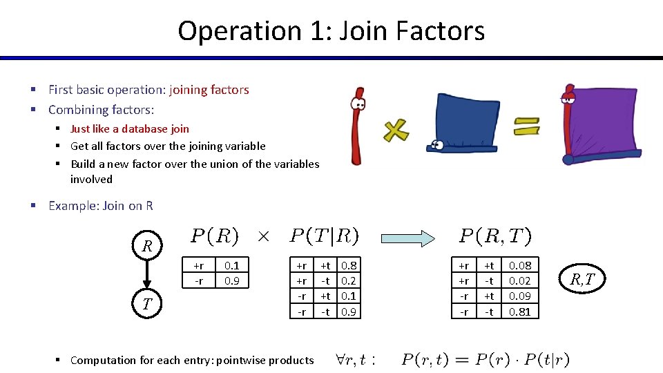
Operation 1: Join Factors § First basic operation: joining factors § Combining factors: § Just like a database join § Get all factors over the joining variable § Build a new factor over the union of the variables involved § Example: Join on R R +r -r T 0. 1 0. 9 +r +r -r -r § Computation for each entry: pointwise products +t -t 0. 8 0. 2 0. 1 0. 9 +r +r -r -r +t -t 0. 08 0. 02 0. 09 0. 81 R, T

Example: Multiple Joins
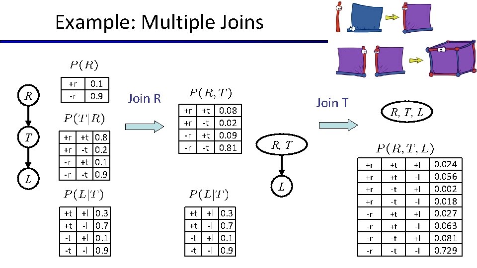
Example: Multiple Joins R T L +r -r +r +r -r -r 0. 1 0. 9 +t -t 0. 8 0. 2 0. 1 0. 9 +t +l 0. 3 +t -l 0. 7 -t +l 0. 1 -t -l 0. 9 Join R +r +t 0. 08 +r -t 0. 02 -r +t 0. 09 -r -t 0. 81 Join T R, T L +t +l 0. 3 +t -l 0. 7 -t +l 0. 1 -t -l 0. 9 R, T, L +r +r -r -r +t +t -t -t +l -l 0. 024 0. 056 0. 002 0. 018 0. 027 0. 063 0. 081 0. 729
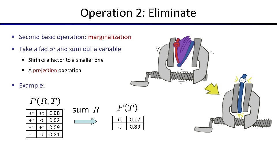
Operation 2: Eliminate § Second basic operation: marginalization § Take a factor and sum out a variable § Shrinks a factor to a smaller one § A projection operation § Example: +r +t 0. 08 +r -t 0. 02 -r +t 0. 09 -r -t 0. 81 +t -t 0. 17 0. 83

Multiple Elimination R, T, L +r +r -r -r +t +t -t -t +l -l T, L 0. 024 0. 056 0. 002 0. 018 0. 027 0. 063 0. 081 0. 729 Sum out R L Sum out T +t +l 0. 051 +t -l 0. 119 -t +l 0. 083 -t -l 0. 747 +l -l 0. 134 0. 866

Thus Far: Multiple Join, Multiple Eliminate (= Inference by Enumeration)

Inference by Enumeration § General case: § We want: § Evidence variables: § Query* variable: § Hidden variables: § Step 1: Select the entries consistent with the evidence * Works fine with multiple query variables, too All variables § Step 2: Sum out H to get joint of Query and evidence § Compute joint § Sum out hidden variables § Step 3: Normalize
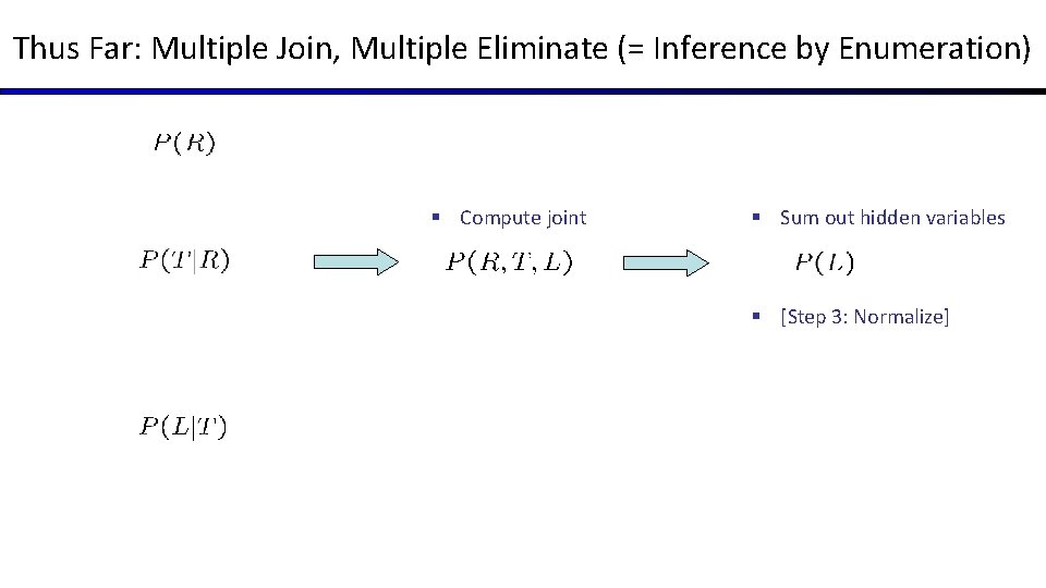
Thus Far: Multiple Join, Multiple Eliminate (= Inference by Enumeration) § Compute joint § Sum out hidden variables § [Step 3: Normalize]

Thus Far: Multiple Join, Multiple Eliminate (= Inference by Enumeration)

Inference by Enumeration vs. Variable Elimination § Why is inference by enumeration so slow? § You join up the whole joint distribution before you sum out the hidden variables § Idea: interleave joining and marginalizing! § Called “Variable Elimination” § Still NP-hard, but usually much faster than inference by enumeration

Traffic Domain R T § Inference by Enumeration § Variable Elimination L Join on r Join on t Eliminate r Eliminate t Eliminate r Join on t Eliminate t

Marginalizing Early (= Variable Elimination)
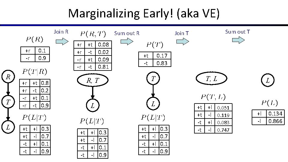
Marginalizing Early! (aka VE) Join R +r -r R T L +r +r -r -r 0. 1 0. 9 +t -t 0. 8 0. 2 0. 1 0. 9 +t +l 0. 3 +t -l 0. 7 -t +l 0. 1 -t -l 0. 9 Sum out R +r +t 0. 08 +r -t 0. 02 -r +t 0. 09 -r -t 0. 81 +t -t 0. 17 0. 83 R, T T L L +t +l 0. 3 +t -l 0. 7 -t +l 0. 1 -t -l 0. 9 Sum out T Join T +t +l 0. 3 +t -l 0. 7 -t +l 0. 1 -t -l 0. 9 T, L +t +l 0. 051 +t -l 0. 119 -t +l 0. 083 -t -l 0. 747 L +l -l 0. 134 0. 866

Evidence § If evidence, start with factors that select that evidence § No evidence uses these initial factors: +r -r 0. 1 0. 9 +r +r -r -r § Computing +r 0. 1 +t -t 0. 8 0. 2 0. 1 0. 9 +t +t -t -t +l -l 0. 3 0. 7 0. 1 0. 9 , the initial factors become: +r +r +t -t 0. 8 0. 2 +t +t -t -t +l -l 0. 3 0. 7 0. 1 0. 9 § We eliminate all vars other than query + evidence

Evidence II § Result will be a selected joint of query and evidence § E. g. for P(L | +r), we would end up with: Normalize +r +l +r -l 0. 026 0. 074 § To get our answer, just normalize this! § That ’s it! +l -l 0. 26 0. 74
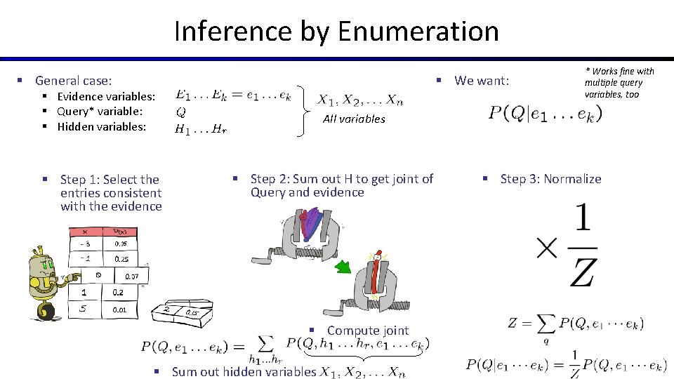
Inference by Enumeration § General case: § We want: § Evidence variables: § Query* variable: § Hidden variables: § Step 1: Select the entries consistent with the evidence * Works fine with multiple query variables, too All variables § Step 2: Sum out H to get joint of Query and evidence § Compute joint § Sum out hidden variables § Step 3: Normalize

Variable Elimination § General case: § We want: § Evidence variables: § Query* variable: § Hidden variables: § Step 1: Select the entries consistent with the evidence * Works fine with multiple query variables, too All variables § Step 2: Sum out H to get joint of Query and evidence § Interleave joining and summing out § Step 3: Normalize
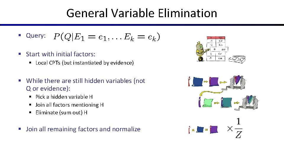
General Variable Elimination § Query: § Start with initial factors: § Local CPTs (but instantiated by evidence) § While there are still hidden variables (not Q or evidence): § Pick a hidden variable H § Join all factors mentioning H § Eliminate (sum out) H § Join all remaining factors and normalize
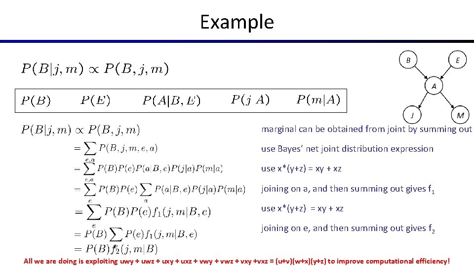
Example marginal can be obtained from joint by summing out use Bayes’ net joint distribution expression use x*(y+z) = xy + xz joining on a, and then summing out gives f 1 use x*(y+z) = xy + xz joining on e, and then summing out gives f 2 All we are doing is exploiting uwy + uwz + uxy + uxz + vwy + vwz + vxy +vxz = (u+v)(w+x)(y+z) to improve computational efficiency!
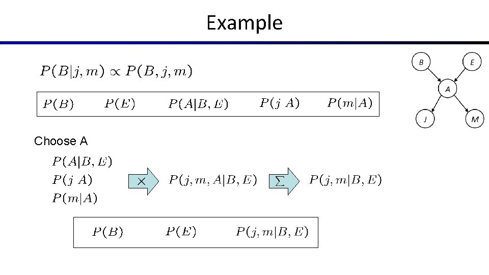
Example Choose A

Example Choose E Finish with B Normalize
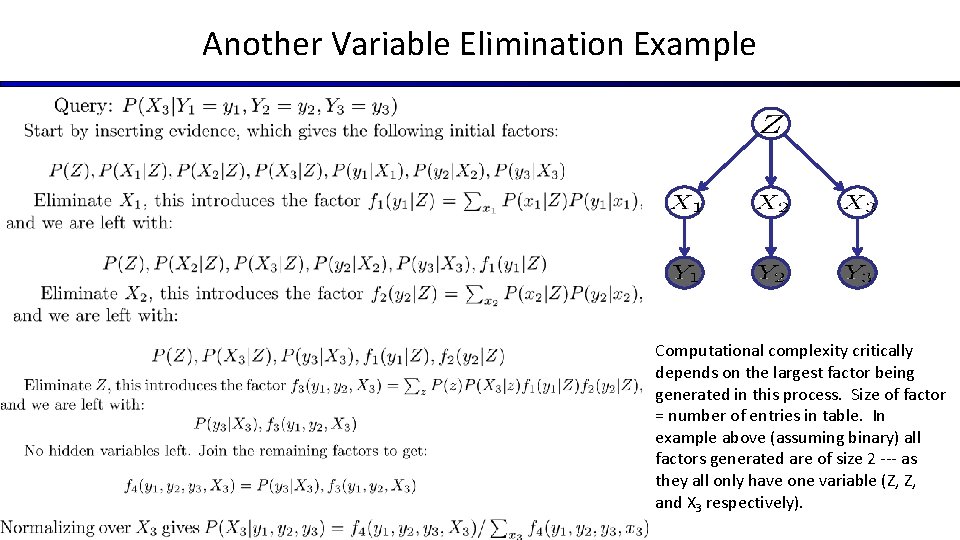
Another Variable Elimination Example Computational complexity critically depends on the largest factor being generated in this process. Size of factor = number of entries in table. In example above (assuming binary) all factors generated are of size 2 --- as they all only have one variable (Z, Z, and X 3 respectively).
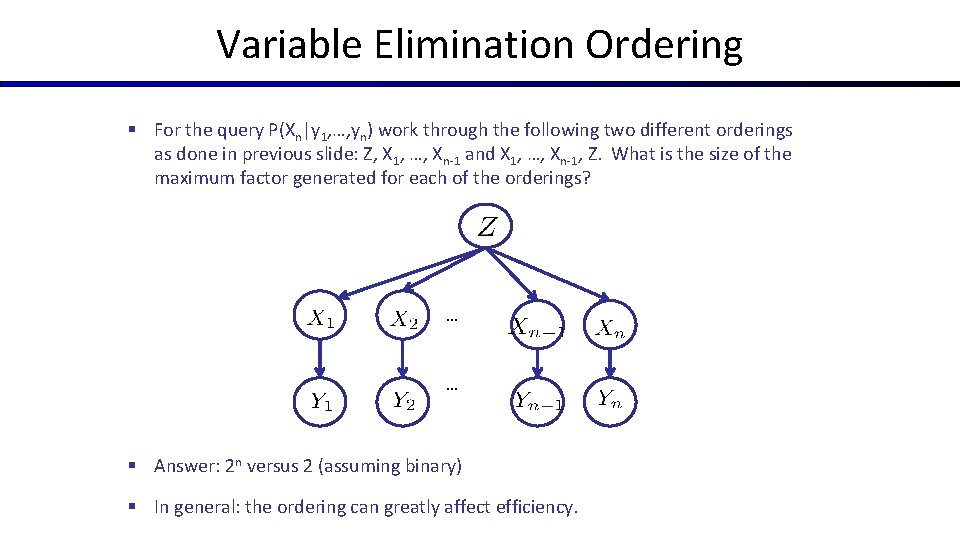
Variable Elimination Ordering § For the query P(Xn|y 1, …, yn) work through the following two different orderings as done in previous slide: Z, X 1, …, Xn-1 and X 1, …, Xn-1, Z. What is the size of the maximum factor generated for each of the orderings? … … § Answer: 2 n versus 2 (assuming binary) § In general: the ordering can greatly affect efficiency.
VE: Computational and Space Complexity § The computational and space complexity of variable elimination is determined by the largest factor § The elimination ordering can greatly affect the size of the largest factor. § E. g. , previous slide’s example 2 n vs. 2 § Does there always exist an ordering that only results in small factors? § No!
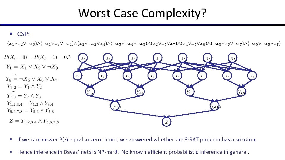
Worst Case Complexity? § CSP: … … § If we can answer P(z) equal to zero or not, we answered whether the 3 -SAT problem has a solution. § Hence inference in Bayes’ nets is NP-hard. No known efficient probabilistic inference in general.
“Easy” Structures: Polytrees § A polytree is a directed graph with no undirected cycles § For poly-trees you can always find an ordering that is efficient § Try it!!
Bayes Nets § Representation § Probabilistic Inference § Enumeration (exact, exponential complexity) § Variable elimination (exact, worst-case exponential complexity, often better) § Probabilistic inference is NP-complete § Conditional Independences § Sampling § Learning from data
- Slides: 38