12 1 Inference for Linear Regression Section 12

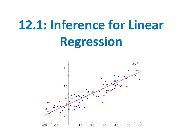
12. 1: Inference for Linear Regression

Section 12. 1 Inference for Linear Regression ü CHECK conditions for performing inference about the slope β of the population regression line ü CONSTRUCT and INTERPRET a confidence interval for the slope β of the population regression line ü PERFORM a significance test about the slope β of a population regression line ü INTERPRET computer output from a least-squares regression analysis

Introduction When a scatterplot shows a linear relationship between a quantitative explanatory variable x and a quantitative response variable y, we can use the leastsquares line fitted to the data to predict y for a given value of x. If the data are a random sample from a larger population, we need statistical inference to answer questions like these: • Is there really a linear relationship between x and y in the population, or could the pattern we see in the scatterplot plausibly happen just by chance? • In the population, how much will the predicted value of y change for each increase of 1 unit in x? What’s the margin of error for this estimate?

Review: General Form of Linear Regression Equation y = a + bx y = dependent variable a = intercept b = slope x = independent variable

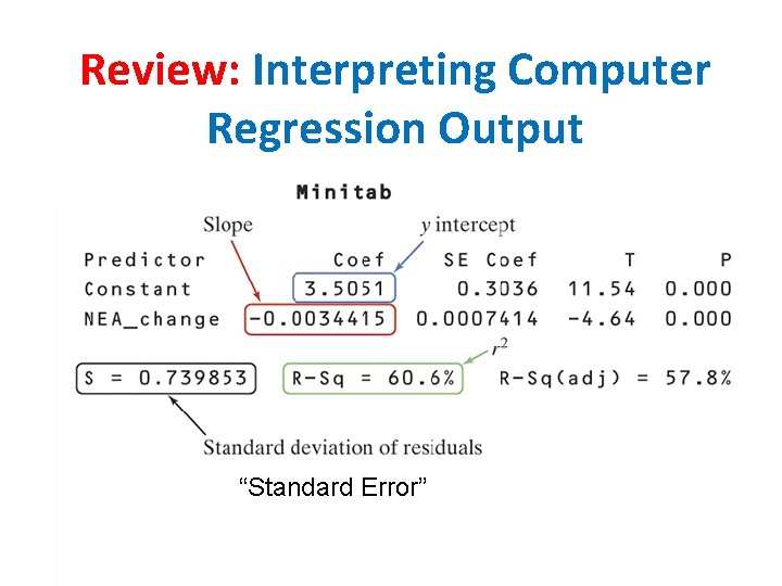
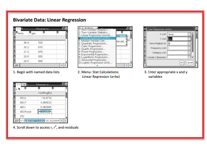
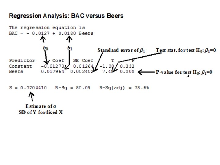
Review: Interpreting Computer Regression Output “Standard Error”

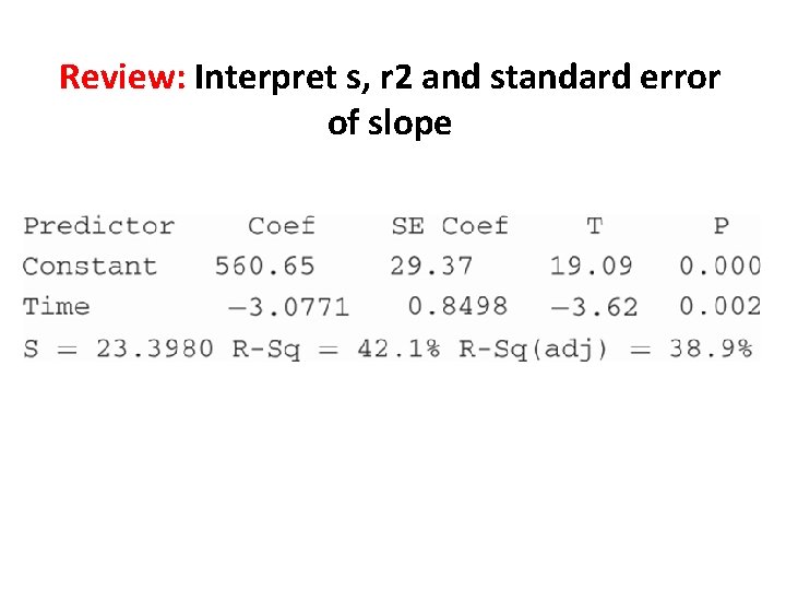
Review: Interpret s, r 2 and standard error of slope

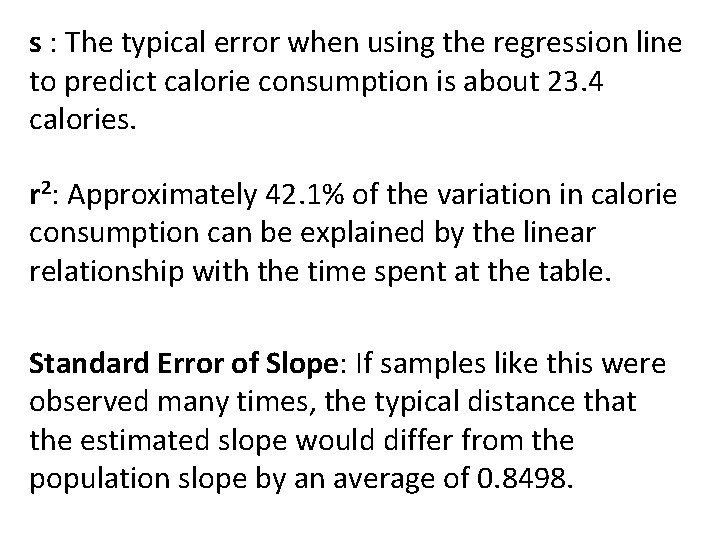
s : The typical error when using the regression line to predict calorie consumption is about 23. 4 calories. r 2: Approximately 42. 1% of the variation in calorie consumption can be explained by the linear relationship with the time spent at the table. Standard Error of Slope: If samples like this were observed many times, the typical distance that the estimated slope would differ from the population slope by an average of 0. 8498.

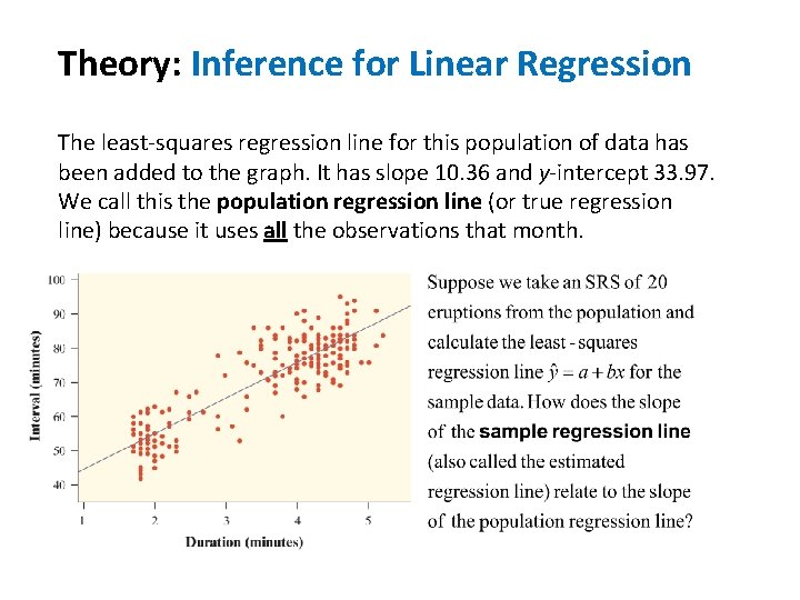
Theory: Inference for Linear Regression The least-squares regression line for this population of data has been added to the graph. It has slope 10. 36 and y-intercept 33. 97. We call this the population regression line (or true regression line) because it uses all the observations that month.

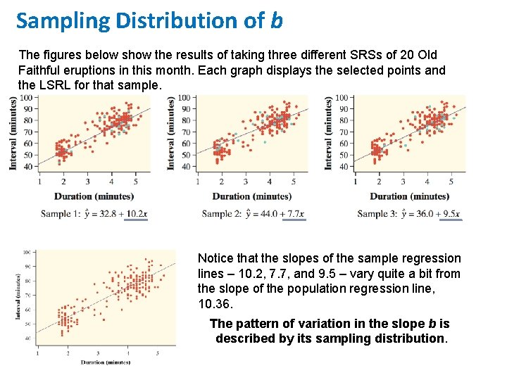
Sampling Distribution of b The figures below show the results of taking three different SRSs of 20 Old Faithful eruptions in this month. Each graph displays the selected points and the LSRL for that sample. Notice that the slopes of the sample regression lines – 10. 2, 7. 7, and 9. 5 – vary quite a bit from the slope of the population regression line, 10. 36. The pattern of variation in the slope b is described by its sampling distribution.

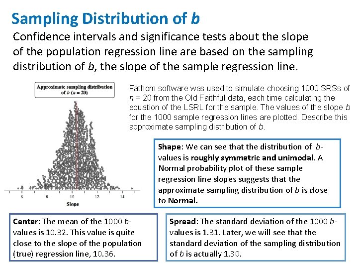
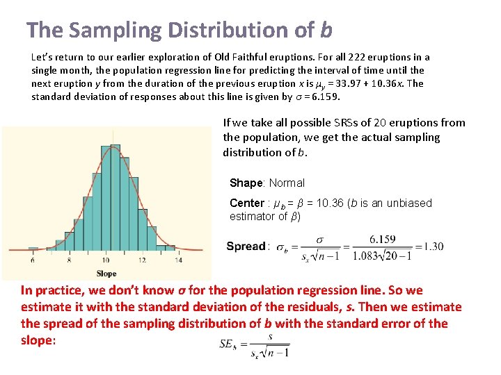
Sampling Distribution of b Confidence intervals and significance tests about the slope of the population regression line are based on the sampling distribution of b, the slope of the sample regression line. Fathom software was used to simulate choosing 1000 SRSs of n = 20 from the Old Faithful data, each time calculating the equation of the LSRL for the sample. The values of the slope b for the 1000 sample regression lines are plotted. Describe this approximate sampling distribution of b. Shape: We can see that the distribution of bvalues is roughly symmetric and unimodal. A Normal probability plot of these sample regression line slopes suggests that the approximate sampling distribution of b is close to Normal. Center: The mean of the 1000 bvalues is 10. 32. This value is quite close to the slope of the population (true) regression line, 10. 36. Spread: The standard deviation of the 1000 bvalues is 1. 31. Later, we will see that the standard deviation of the sampling distribution of b is actually 1. 30.

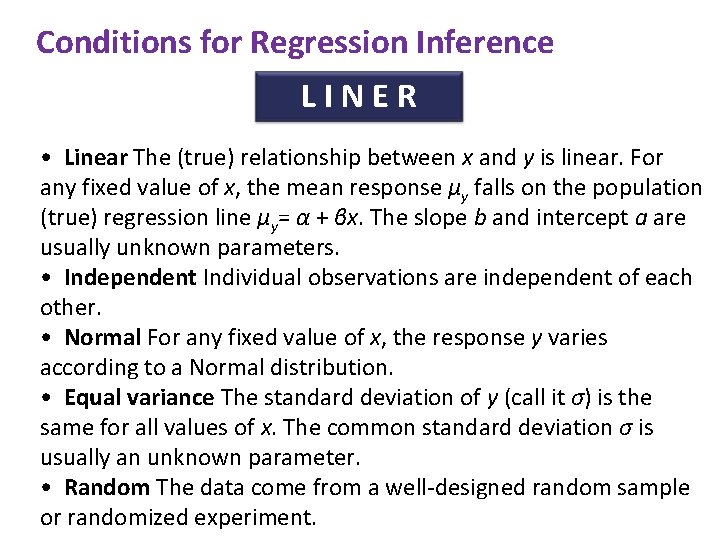
Conditions for Regression Inference LINER • Linear The (true) relationship between x and y is linear. For any fixed value of x, the mean response µy falls on the population (true) regression line µy= α + βx. The slope b and intercept a are usually unknown parameters. • Independent Individual observations are independent of each other. • Normal For any fixed value of x, the response y varies according to a Normal distribution. • Equal variance The standard deviation of y (call it σ) is the same for all values of x. The common standard deviation σ is usually an unknown parameter. • Random The data come from a well-designed random sample or randomized experiment.

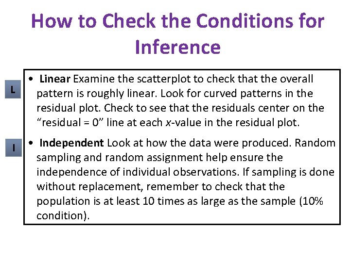
How to Check the Conditions for Inference L I • Linear Examine the scatterplot to check that the overall pattern is roughly linear. Look for curved patterns in the residual plot. Check to see that the residuals center on the “residual = 0” line at each x-value in the residual plot. • Independent Look at how the data were produced. Random sampling and random assignment help ensure the independence of individual observations. If sampling is done without replacement, remember to check that the population is at least 10 times as large as the sample (10% condition).

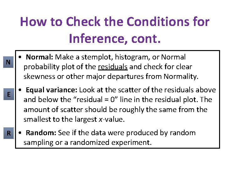
How to Check the Conditions for Inference, cont. • Normal: Make a stemplot, histogram, or Normal N probability plot of the residuals and check for clear skewness or other major departures from Normality. • Equal variance: Look at the scatter of the residuals above E and below the “residual = 0” line in the residual plot. The amount of scatter should be roughly the same from the smallest to the largest x-value. R • Random: See if the data were produced by random sampling or a randomized experiment.

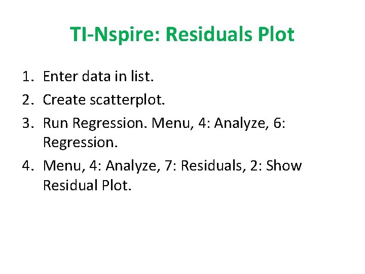
TI-Nspire: Residuals Plot 1. Enter data in list. 2. Create scatterplot. 3. Run Regression. Menu, 4: Analyze, 6: Regression. 4. Menu, 4: Analyze, 7: Residuals, 2: Show Residual Plot.

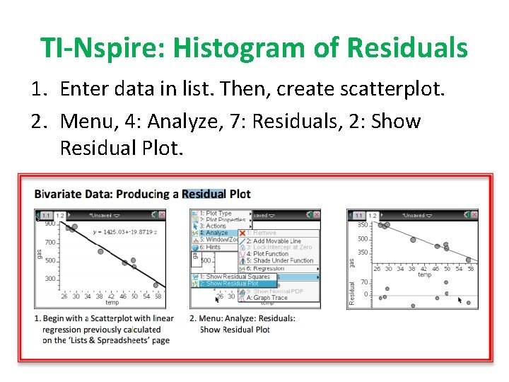
TI-Nspire: Histogram of Residuals 1. Enter data in list. Then, create scatterplot. 2. Menu, 4: Analyze, 7: Residuals, 2: Show Residual Plot.

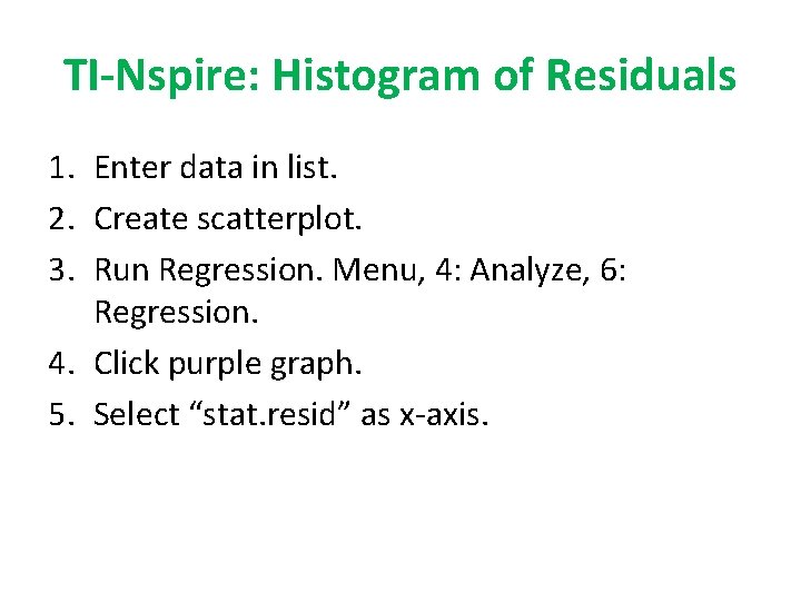
TI-Nspire: Histogram of Residuals 1. Enter data in list. 2. Create scatterplot. 3. Run Regression. Menu, 4: Analyze, 6: Regression. 4. Click purple graph. 5. Select “stat. resid” as x-axis.

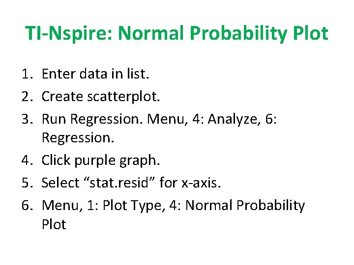
TI-Nspire: Normal Probability Plot 1. Enter data in list. 2. Create scatterplot. 3. Run Regression. Menu, 4: Analyze, 6: Regression. 4. Click purple graph. 5. Select “stat. resid” for x-axis. 6. Menu, 1: Plot Type, 4: Normal Probability Plot

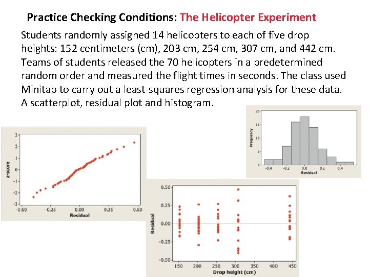
Practice Checking Conditions: The Helicopter Experiment Students randomly assigned 14 helicopters to each of five drop heights: 152 centimeters (cm), 203 cm, 254 cm, 307 cm, and 442 cm. Teams of students released the 70 helicopters in a predetermined random order and measured the flight times in seconds. The class used Minitab to carry out a least-squares regression analysis for these data. A scatterplot, residual plot and histogram.

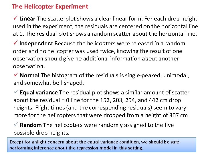
The Helicopter Experiment ü Linear The scatterplot shows a clear linear form. For each drop height used in the experiment, the residuals are centered on the horizontal line at 0. The residual plot shows a random scatter about the horizontal line. ü Independent Because the helicopters were released in a random order and no helicopter was used twice, knowing the result of one observation should give no additional information about another observation. ü Normal The histogram of the residuals is single-peaked, unimodal, and somewhat bell-shaped. ü Equal variance The residual plot shows a similar amount of scatter about the residual = 0 line for the 152, 203, 254, and 442 cm drop heights. Flight times (and the corresponding residuals) seem to vary more for the helicopters that were dropped from a height of 307 cm. ü Random The helicopters were randomly assigned to the five possible drop heights. Except for a slight concern about the equal-variance condition, we should be safe performing inference about the regression model in this setting.

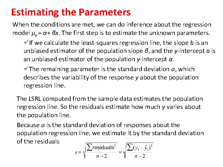
Estimating the Parameters When the conditions are met, we can do inference about the regression model µy = α+ βx. The first step is to estimate the unknown parameters. üIf we calculate the least-squares regression line, the slope b is an unbiased estimator of the population slope β, and the y-intercept a is an unbiased estimator of the population y-intercept α. üThe remaining parameter is the standard deviation σ, which describes the variability of the response y about the population regression line. The LSRL computed from the sample data estimates the population regression line. So the residuals estimate how much y varies about the population line. Because σ is the standard deviation of responses about the population regression line, we estimate it by the standard deviation of the residuals

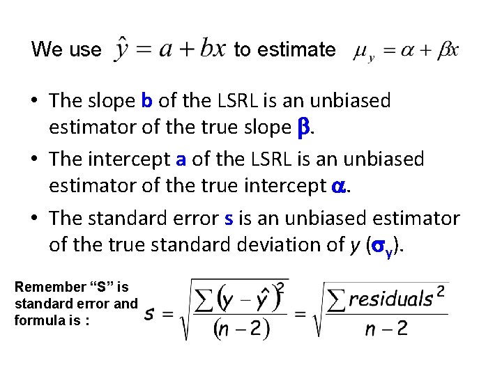
We use to estimate • The slope b of the LSRL is an unbiased estimator of the true slope b. • The intercept a of the LSRL is an unbiased estimator of the true intercept a. • The standard error s is an unbiased estimator of the true standard deviation of y (sy). Remember “S” is standard error and formula is :

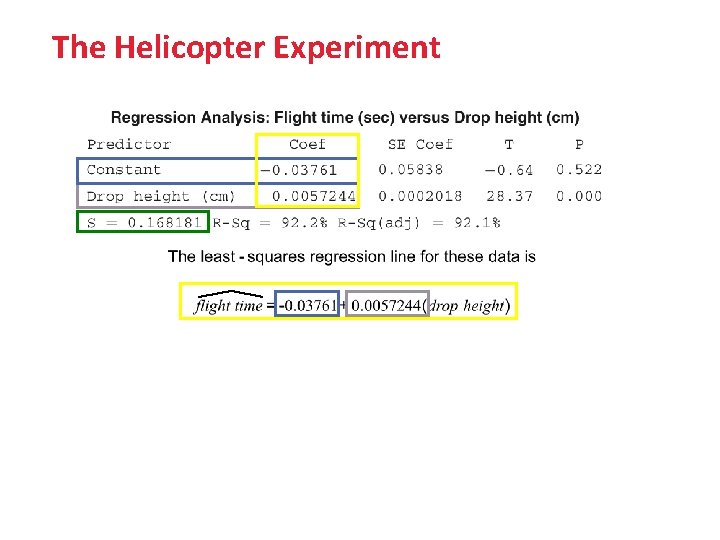
The Helicopter Experiment

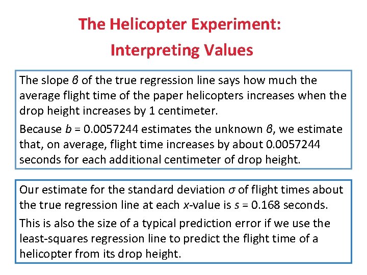
The Helicopter Experiment: Interpreting Values The slope β of the true regression line says how much the average flight time of the paper helicopters increases when the drop height increases by 1 centimeter. Because b = 0. 0057244 estimates the unknown β, we estimate that, on average, flight time increases by about 0. 0057244 seconds for each additional centimeter of drop height. Our estimate for the standard deviation σ of flight times about the true regression line at each x-value is s = 0. 168 seconds. This is also the size of a typical prediction error if we use the least-squares regression line to predict the flight time of a helicopter from its drop height.

The Helicopter Experiment: Interpreting Values We need the intercept a = -0. 03761 to draw the line and make predictions, but it has no statistical meaning in this example. No helicopter was dropped from less than 150 cm, so we have no data near x = 0. We might expect the actual y-intercept α of the true regression line to be 0 because it should take no time for a helicopter to fall no distance. The y-intercept of the sample regression line is -0. 03761, which is pretty close to 0.

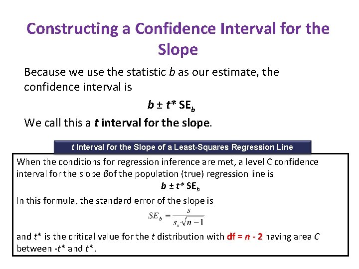
Constructing a Confidence Interval for the Slope Because we use the statistic b as our estimate, the confidence interval is b ± t* SEb We call this a t interval for the slope. t Interval for the Slope of a Least-Squares Regression Line When the conditions for regression inference are met, a level C confidence interval for the slope βof the population (true) regression line is b ± t* SEb In this formula, the standard error of the slope is and t* is the critical value for the t distribution with df = n - 2 having area C between -t* and t*.

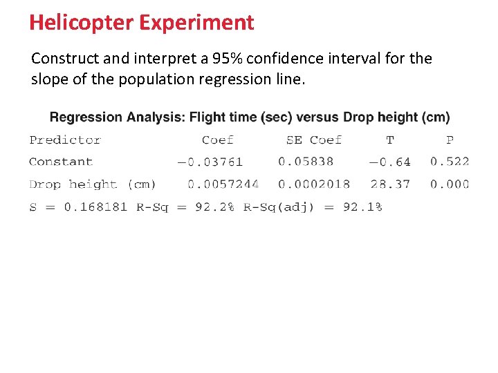
Helicopter Experiment Construct and interpret a 95% confidence interval for the slope of the population regression line.

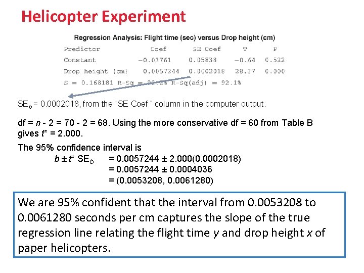
Helicopter Experiment SEb = 0. 0002018, from the “SE Coef ” column in the computer output. df = n - 2 = 70 - 2 = 68. Using the more conservative df = 60 from Table B gives t* = 2. 000. The 95% confidence interval is b ± t* SEb = 0. 0057244 ± 2. 000(0. 0002018) = 0. 0057244 ± 0. 0004036 = (0. 0053208, 0. 0061280) We are 95% confident that the interval from 0. 0053208 to 0. 0061280 seconds per cm captures the slope of the true regression line relating the flight time y and drop height x of paper helicopters.

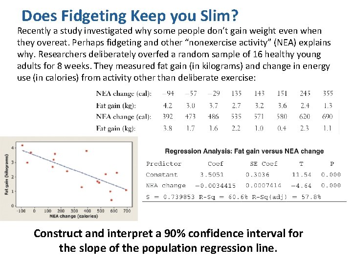
Does Fidgeting Keep you Slim? Recently a study investigated why some people don’t gain weight even when they overeat. Perhaps fidgeting and other “nonexercise activity” (NEA) explains why. Researchers deliberately overfed a random sample of 16 healthy young adults for 8 weeks. They measured fat gain (in kilograms) and change in energy use (in calories) from activity other than deliberate exercise: Construct and interpret a 90% confidence interval for the slope of the population regression line.

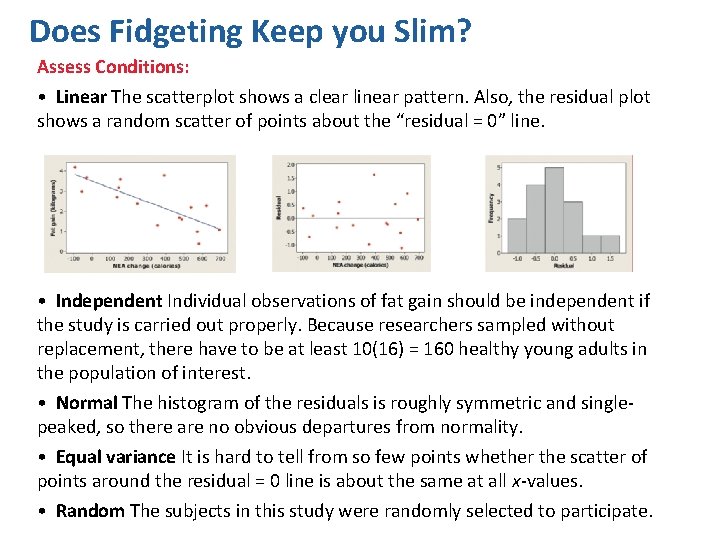
Does Fidgeting Keep you Slim? Assess Conditions: • Linear The scatterplot shows a clear linear pattern. Also, the residual plot shows a random scatter of points about the “residual = 0” line. • Independent Individual observations of fat gain should be independent if the study is carried out properly. Because researchers sampled without replacement, there have to be at least 10(16) = 160 healthy young adults in the population of interest. • Normal The histogram of the residuals is roughly symmetric and singlepeaked, so there are no obvious departures from normality. • Equal variance It is hard to tell from so few points whether the scatter of points around the residual = 0 line is about the same at all x-values. • Random The subjects in this study were randomly selected to participate.

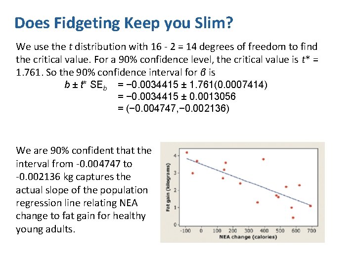
Does Fidgeting Keep you Slim? We use the t distribution with 16 - 2 = 14 degrees of freedom to find the critical value. For a 90% confidence level, the critical value is t* = 1. 761. So the 90% confidence interval for β is b ± t* SEb = − 0. 0034415 ± 1. 761(0. 0007414) = − 0. 0034415 ± 0. 0013056 = (− 0. 004747, − 0. 002136) We are 90% confident that the interval from -0. 004747 to -0. 002136 kg captures the actual slope of the population regression line relating NEA change to fat gain for healthy young adults.

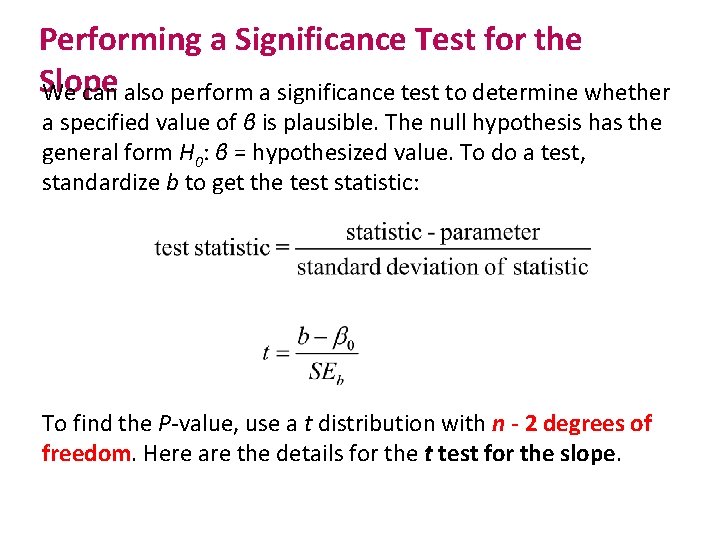
Performing a Significance Test for the Slope We can also perform a significance test to determine whether a specified value of β is plausible. The null hypothesis has the general form H 0: β = hypothesized value. To do a test, standardize b to get the test statistic: To find the P-value, use a t distribution with n - 2 degrees of freedom. Here are the details for the t test for the slope.

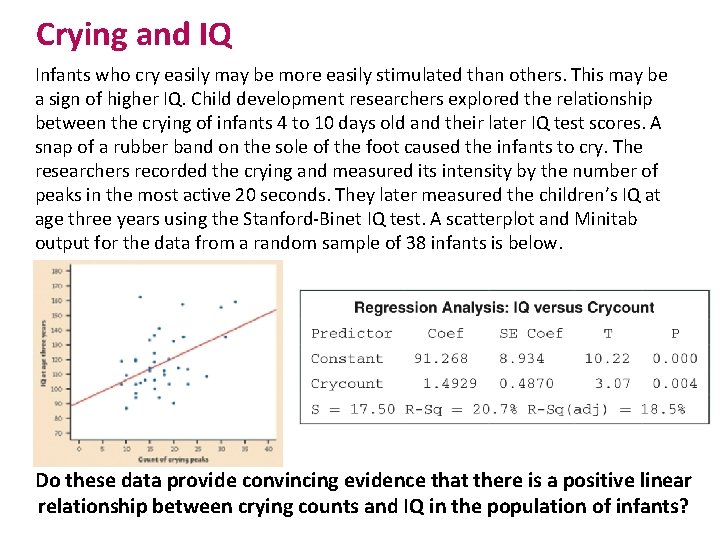
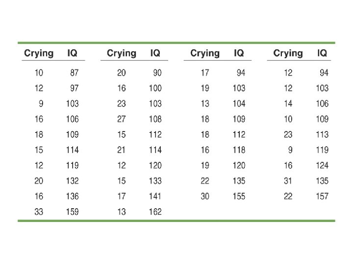
Crying and IQ Infants who cry easily may be more easily stimulated than others. This may be a sign of higher IQ. Child development researchers explored the relationship between the crying of infants 4 to 10 days old and their later IQ test scores. A snap of a rubber band on the sole of the foot caused the infants to cry. The researchers recorded the crying and measured its intensity by the number of peaks in the most active 20 seconds. They later measured the children’s IQ at age three years using the Stanford-Binet IQ test. A scatterplot and Minitab output for the data from a random sample of 38 infants is below. Do these data provide convincing evidence that there is a positive linear relationship between crying counts and IQ in the population of infants?

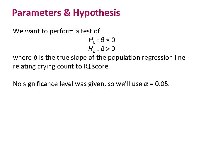
Parameters & Hypothesis We want to perform a test of H 0 : β = 0 Ha : β > 0 where β is the true slope of the population regression line relating crying count to IQ score. No significance level was given, so we’ll use α = 0. 05.

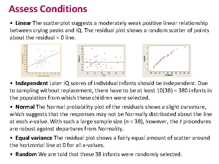
Assess Conditions • Linear The scatterplot suggests a moderately weak positive linear relationship between crying peaks and IQ. The residual plot shows a random scatter of points about the residual = 0 line. • Independent Later IQ scores of individual infants should be independent. Due to sampling without replacement, there have to be at least 10(38) = 380 infants in the population from which these children were selected. • Normal The Normal probability plot of the residuals shows a slight curvature, which suggests that the responses may not be Normally distributed about the line at each x-value. With such a large sample size (n = 38), however, the t procedures are robust against departures from Normality. • Equal variance The residual plot shows a fairly equal amount of scatter around the horizontal line at 0 for all x-values. • Random We are told that these 38 infants were randomly selected.

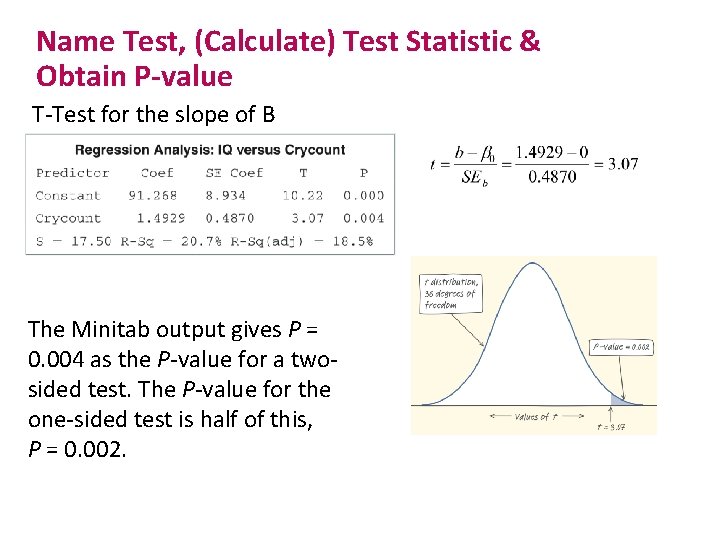
Name Test, (Calculate) Test Statistic & Obtain P-value T-Test for the slope of B The Minitab output gives P = 0. 004 as the P-value for a twosided test. The P-value for the one-sided test is half of this, P = 0. 002.

Make Decision & State Conclusion The P-value, 0. 002, is less than our α = 0. 05 significance level, so we have enough evidence to reject H 0 and conclude that there is a positive linear relationship between intensity of crying and IQ score in the population of infants.

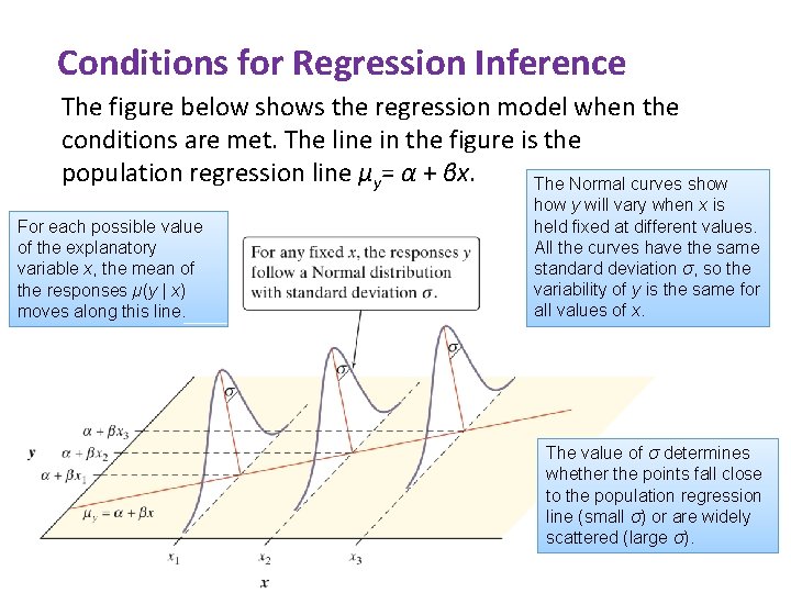
Conditions for Regression Inference The figure below shows the regression model when the conditions are met. The line in the figure is the population regression line µy= α + βx. The Normal curves show For each possible value of the explanatory variable x, the mean of the responses µ(y | x) moves along this line. how y will vary when x is held fixed at different values. All the curves have the same standard deviation σ, so the variability of y is the same for all values of x. The value of σ determines whether the points fall close to the population regression line (small σ) or are widely scattered (large σ).

The Sampling Distribution of b Let’s return to our earlier exploration of Old Faithful eruptions. For all 222 eruptions in a single month, the population regression line for predicting the interval of time until the next eruption y from the duration of the previous eruption x is µy = 33. 97 + 10. 36 x. The standard deviation of responses about this line is given by σ = 6. 159. If we take all possible SRSs of 20 eruptions from the population, we get the actual sampling distribution of b. Shape: Normal Center : µb = β = 10. 36 (b is an unbiased estimator of β) In practice, we don’t know σ for the population regression line. So we estimate it with the standard deviation of the residuals, s. Then we estimate the spread of the sampling distribution of b with the standard error of the slope:

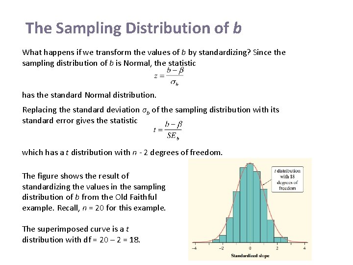
The Sampling Distribution of b What happens if we transform the values of b by standardizing? Since the sampling distribution of b is Normal, the statistic has the standard Normal distribution. Replacing the standard deviation σb of the sampling distribution with its standard error gives the statistic which has a t distribution with n - 2 degrees of freedom. The figure shows the result of standardizing the values in the sampling distribution of b from the Old Faithful example. Recall, n = 20 for this example. The superimposed curve is a t distribution with df = 20 – 2 = 18.