Synchronous Computations Chapter 6 o In this chapter

Synchronous Computations Chapter 6

o In this chapter, we will consider problems solved by a group of separate computations that must at times wait for each other before proceeding. n n A very important class of such applications is called fully synchronous applications. o All processes are synchronized at regular points. (Similar to SIMD structure) First we will consider synchronizing processes and then fully synchronous applications.

1. Synchronization o 1. 1 Barrier n n A basic mechanism for synchronizing processes - inserted at the point in each process where it must wait. All processes can continue from this point when all the processes have reached it (or, in some implementations, when a stated number of processes have reached this point).

1. 1 Barrier

1. 1 Barrier n Barriers apply to both shared memory and message-passing systems. In messagepassing systems barriers are often provided with library routines.

1. 1 Barrier n MPI o o MPI_Barrier() - barrier with a named communicator being the only parameter. Called by each process in the group, blocking until all members of the group have reached the barrier call and only returning then.

1. 1 Barrier n n n As usual, MPI does not specify the internal implementation. However, we need to know something about the implementation to assess the complexity of the barrier. So, let us review some of the common implementations of a barrier.

1. 2 Counter Implementation o Sometimes called a Linear Barrier

1. 2 Counter Implementation n Counter-based barriers often have two phases: o o A process enters arrival phase and does not leave this phase until all processes have arrived in this phase. Then processes move to departure phase and are released.

1. 2 Counter Implementation n Good implementations of a barrier must take into account that a barrier might be used more than once in a process. o o It might be possible for a process to enter the barrier for a second time before previous processes have left the barrier for the first time. The two phases above handle this scenario.

1. 2 Counter Implementation n Example code: o Master: for (i = 0; i < n; i++) /*count slaves as they reach barrier*/ recv(P any ); for (i = 0; i < n; i++) /* release slaves */ send(P i ); o Slave processes: send(P master ); recv(P master );

1. 2 Counter Implementation n The complete arrangement is illustrated here

1. 3 Tree Implementation n More efficient. o n Suppose there are eight processes, o n O(log p) steps P 0 , P 1 , P 2 , P 3 , P 4 , P 5 , P 6 , and P 7 : First stage: o o P P 1 3 5 7 sends message to to P P 0 2 4 6 ; ; (when P P 1 3 5 7 reaches its its barrier)

1. 3 Tree Implementation n Second stage: o P 2 sends message to P 0 ; n o P 6 sends message to P 4 ; n n (P 6 and P 7 have reached their barrier) Third stage: o P 4 sends message to P 0 ; n o (P 4 , P 5 , P 6 , and P 7 have reached their barrier) P 0 terminates arrival phase; n n (P 2 and P 3 have reached their barrier) (when P 0 reaches barrier and has received message from P 4 ) Release with a reverse tree construction.

1. 3 Tree Implementation

1. 4 Butterfly Barrier o o o First stage n P 0 « P 1, P 2 « P 3, P 4 « P 5, P 6 « P 7 Second stage n P 0 « P 2, P 1 « P 3, P 4 « P 6, P 5 « P 7 Third stage n P 0 « P 4, P 1 « P 5, P 2 « P 6, P 3 « P 7

1. 5 Local Synchronization n Suppose a process Pi needs to be synchronized and to exchange data with process Pi-1 and process Pi+1 before continuing: Process Pi-1 recv(P i ); send(P i ); recv(P i-1 ); n Process Pi send(P i-1 ); send(P i+1 ); Process Pi+1 recv(P i ); send(P i ); recv(P i+1 ); Not a perfect three-process barrier because o process Pi-1 will only synchronize with Pi and continue as soon as Pi allows. o Similarly, process Pi+1 only synchronizes with Pi.

1. 6 Deadlock n n When a pair of processes each send and receive from each other, deadlock may occur. Deadlock will occur if both processes perform the send, using synchronous routines first (or blocking routines without sufficient buffering). This is because neither will return; they will wait for matching receives that are never reached.

1. 6 Deadlock n A Solution o n Arrange for one process to receive first and then send and the other process to send first and then receive. Example o Linear pipeline, deadlock can be avoided by arranging so the even-numbered processes perform their sends first and the oddnumbered processes perform their receives first.

1. 6 Deadlock n n Combined deadlock-free blocking sendrecv() routines o MPI provides routine MPI_Sendrecv() and MPI_Sendrecv_replace(). Example Process Pi-1 Process Pi+1 sendrecv(P i ); sendrecv(P i-1 ); sendrecv(P i+1 ); sendrecv(P i ); n Please note that MPI_Sendrecv has 12 parameters o essentially a concatenation of the parameter list for MPI_Send() and MPI_Recv()

2. Synchronized Computations o Can be classififed as: n n o o Fully synchronous or Locally synchronous In fully synchronous, all processes involved in the computation must be synchronized. In locally synchronous, processes only need to synchronize with a set of logically nearby processes, not all processes involved in the computation

2. 1 Data Parallel Computations n n n Fully Synchronous Same operation performed on different data elements simultaneously; i. e. , in parallel. Particularly convenient because: o o o Ease of programming (essentially one program). Can scale easily to larger problem sizes. Many numeric and some non-numeric problems can be cast in a data parallel form.

2. 1 Data Parallel Computations n Example o To add the same constant to each element of an array: for (i = 0; i < n; i++) a[i] = a[i] + k; o The statement a[i] = a[i] + k could be executed simultaneously by multiple processors, each using a different index i (0 < i £ n).

2. 1 Data Parallel Computations n Forall construct o Special “parallel” construct in parallel programming languages to specify data parallel operations o Example forall (i = 0; i < n; i++) { body } o o states that n instances of the statements of the body can be executed simultaneously. One value of the loop variable i is valid in each instance of the body, the first instance has i = 0, the next i = 1, and so on. n (Think of this as loop unrolling across processors)

2. 1 Data Parallel Computations o To add k to each element of an array, a, we can write forall (i = 0; i < n; i++) a[i] = a[i] + k; n Data parallel technique applied to multiprocessors and multicomputers - Example: o To add k to the elements of an array: i = myrank; a[i] = a[i] + k; /* body */ barrier(mygroup); o where myrank is a process rank between 0 and n 1.

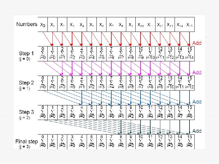
2. 1 Data Parallel Computations n Prefix Sum Problem o Given a list of numbers, n o compute all the partial summations n o o o x 0, …, xn-1 , (i. e. , x 0+x 1; x 0+x 1+x 2+x 3; … ). Can also be defined with associative operations other than addition. Widely studied. Practical applications in areas such as processor allocation, data compaction, sorting, and polynomial evaluation.

2. 1 Data Parallel Computations o o The sequential code for the prefix problem could be for(i = 0; i < n; i++) { sum[i] = 0; for (j = 0; j <= i; j++) sum[i] = sum[i] + x[j]; } This is an O(n 2) algorithm.

2. 1 Data Parallel Computations n Data parallel method of adding all partial sums of 16 numbers o Sequential code for (j = 0; j < log(n); j++)/* at each step */ for (i = 2 j; i < n; i++)/*add to accum. sum */ x[i] = x[i] + x[i - 2 j]; o Written up by Hillis and Steel (1986) n requires a different number of computations at each step.

2. 1 Data Parallel Computations o o Because SIMD machines must send the same instruction to all processors, you could rewrite it as: Parallel code: for (j = 0; j < log(n); j++)/* at each step */ forall (i = 0; i < n; i++)/* add to accum. sum */ if (i >= 2 j) x[i] = x[i] + x[i - 2 j]; o o This uses a maximum of n-1 processors. The time complexity is O(n log n) which is not cost optimal since the sequential was O(n 2)

2. 2 Synchronous Iteration n n Each iteration is composed of several processes o they start together at beginning of iteration o and the next iteration cannot begin until all processes have finished previous iteration. The forall construct could be used to specify the parallel bodies of the synchronous iteration: for (j = 0; j < n; j++) /*for each synch. iteration */ forall (i = 0; i < N; i++) { /*N procs each executing */ body(i); /*using specific value of i */ }

2. 2 Synchronous Iteration n Or it could be written this way: for (j = 0; j<n; j++) {/*for each synchr. iteration*/ i = myrank; /*find value of i to be used */ body(i); /*using specific value of i */ barrier(mygroup); } n Let us look at some specific synchronous iteration examples

3. Synchronous Iteration Program Examples o 3. 1 Solving a System of Linear Equations by Iteration n Suppose the equations are of a general form with n equations and n unknowns where the unknowns are x 0, x 1, x 2, … xn-1 (0 £ i < n). o o o an-1, 0 x 0 + an-1, 1 x 1 + a n-1, 2 x 2 …+ a n-1, n-1 x. . a 2, 0 x 0 + a 2, 1 x 1+ a 2, 2 x 2 … + a 2, n-1 xn-1 = b 2 a 1, 0 x 0 + a 1, 1 x 1+ a 1, 2 x 2 … + a 1, n-1 xn-1 = b 1 a 0, 0 x 0 + a 0, 1 x 1+ a 0, 2 x 2 … + a 0, n-1 xn-1 = b 0 n-1 =b n-1

3. 1 Solving a System of Linear Equations by Iteration n One way to solve these equations for the unknowns is by iteration. By rearranging the ith equation: ai, 0 x 0 + ai, 1 x 1+ a 2, 2 x 2 … + a 2, n-1 xn-1 = b 2 n to xi=(1/ai, i)[bi-(ai, 0 x 0+ai, 1 x 1+ai, 2 x 2 … ai, i -1 xi-1+ai , i+1 xi+1 … +ai, n-1 xn-1)] n n or This equation gives xi in terms of the other unknowns and can be be used as an iteration formula for each of the unknowns to obtain better approximations.

3. 1 Solving a System of Linear Equations by Iteration n Jacobi Iteration o Iterative method described called a Jacobi iteration n o o all values of x are updated together. It can be proven that the Jacobi method will converge if the diagonal values of a have an absolute value greater than the sum of the absolute values of the other a’s on the row(the array of a’s is diagonally dominant) i. e. If This condition is a sufficient but not a necessary condition.

3. 1 Solving a System of Linear Equations by Iteration n Termination o A simple, common approach is to compare values computed in each iteration to the values obtained from the previous iteration, and then to terminate the computation in the tth iteration when all values are within a given tolerance; i. e. , when o o for all i, where xit is the value of xi after the tth iteration and is the value of xit-1 after the (t - 1)th iteration. However, this does not guarantee the solution to that accuracy.

3. 1 Solving a System of Linear Equations by Iteration

3. 1 Solving a System of Linear Equations by Iteration n Sequential Code o Given arrays a[ ][ ] and b[ ] holding constants in the equations, x[ ] holding unknowns, and fixed number of iterations: for (i = 0; i < n; i++) x[i] = b[i]; /*initialize unknowns*/ for (iteration = 0; iteration < limit; iteration++) { for (i = 0; i < n; i++) { /* for each unknown */ sum = 0; for (j = 0; j < n; j++) /* summation of a[][]x[] */ if (i != j) sum = sum + a[i][j] * x[j]; new_x[i] = (b[i] - sum) / a[i][i]; /*compute unknown*/ } for (i = 0; i < n; i++) x[i] = new_x[i]; /* update values */ }

3. 1 Solving a System of Linear Equations by Iteration n Slightly more efficient sequential code: for (i = 0; i < n; i++) x[i] = b[i]; /*initialize unknowns*/ for (iteration = 0; iteration < limit; iteration++) { for (i = 0; i < n; i++) { /* for each unknown */ sum = -a[i][i] * x[i]; for (j = 0; j < n; j++) /* compute summation */ sum = sum + a[i][j] * x[j]; new_x[i] = (b[i] - sum) / a[i][i]; /*compute unknown*/ } for (i = 0; i < n; i++) x[i] = new_x[i]; /*update */ }

3. 1 Solving a System of Linear Equations by Iteration n Parallel Code - Process P i could be of the form x[i] = b[i]; /*initialize unknown*/ for (iteration = 0; iteration < limit; iteration++) { sum = -a[i][i] * x[i]; for (j = 0; j < n; j++) /* compute summation */ sum = sum + a[i][j] * x[j]; new_x[i] = (b[i] - sum) / a[i][i]; /* compute unknown */ broadcast_receive(&new_x[i]); /* broadcast value */ global_barrier(); /* wait for all processes */ } o o broadcast_receive(), sends the newly computed value of x[i] from process i to every other process and collects data broadcast from the other processes. An alternative simple solution is to return to basic send()s and recv()s.

3. 1 Solving a System of Linear Equations by Iteration n Allgather o Broadcast and gather values in one composite construction.

3. 1 Solving a System of Linear Equations by Iteration n Iterate until approximations are sufficiently close: x[i] = b[i]; /*initialize unknown*/ iteration = 0; do { iteration++; sum = -a[i][i] * x[i]; for (j = 1; j < n; j++) /* compute summation */ sum = sum + a[i][j] * x[j]; new_x[i] = (b[i] - sum) / a[i][i]; /* compute unknown */ broadcast_receive(&new_x[i]); /*broadcast value & wait */ } while (tolerance() && (iteration < limit)); n where tolerance() returns FALSE if ready to terminate; otherwise it returns TRUE.

3. 1 Solving a System of Linear Equations by Iteration n Partitioning o Usually the number of processors much fewer than number of data items to be processed. Partition the problem so that processors take on more than one data item.

3. 1 Solving a System of Linear Equations by Iteration n In the problem at hand, each process can be responsible for computing a group of unknowns. n n o block allocation – allocate groups of consecutive unknowns to processors in increasing order. cyclic allocation – processors are allocated one unknown in order; i. e. , processor P 0 is allocated x 0, xp , x 2 p , …, x((n/p)-1)p , processor P 1 is allocated x 1, xp+1, x 2 p+1, …, x((n/p)1)p+1, and so on. Cyclic allocation no particular advantage here n (Indeed, may be disadvantageous because the indices of unknowns have to be computed in a more complex way).

3. 1 Solving a System of Linear Equations by Iteration n Analysis o Suppose there are n equations and p processors. o A processor operates upon n/p unknowns. o Suppose there are t iterations. o One iteration has a computational phase and a broadcast communication phase. n n n o Computation. § tcomp = n/p(2 n + 4)t Communication. § tcomm = p(tstartup+(n/p)tdata)t = (ptstartup+ntdata)t Overall. § tp = (n/p(2 n + 4) + ptstartup+ ntdata)t The resulting total execution time has a minimum value.

3. 1 Solving a System of Linear Equations by Iteration o Effects of computation and communication in Jacobi iteration

3. 2 Heat Distribution Problem n n Locally Synchronous Computation A square metal sheet has known temperatures along each of its edges. o Find the temperature distribution.

3. 2 Heat Distribution Problem n Dividing the area into a fine mesh of points, hi, j. o n The temperature at an inside point can be taken to be the average of the temperatures of the four neighboring points. Convenient to describe the edges by points adjacent to the interior points. o The interior points of hi, j are where 0<i< n, 0< j< n [(n - 1) ´ (n - 1) interior points].

3. 2 Heat Distribution Problem n Temperature of each point by iterating the equation: o o (0 < i < n, 0 < j < n) for a fixed number of iterations or until the difference between iterations of a point is less than some very small prescribed amount.

3. 2 Heat Distribution Problem

3. 2 Heat Distribution Problem o Natural Ordering

3. 2 Heat Distribution Problem n n n Points numbered from 1 for convenience and include those representing the edges. Each point will then use the equation Could be written as a linear equation containing the unknowns x i-k , x i-1 , x i+1 , and x i+k : xi-k+xi-1 -4 x i+xi+1+xi-k= 0 Known as the finite difference method. Also solving Laplace’s equation.

3. 2 Heat Distribution Problem n Sequential Code o Using a fixed number of iterations for (iteration = 0; iteration < limit; iteration++) { for (i = 1; i < n; i++) for (j = 1; j < n; j++) g[i][j] = 0. 25*(h[i-1][j]+h[i+1][j]+h[i][j-1]+h[i][j+1]); for (i = 1; i < n; i++) /* update points */ for (j = 1; j < n; j++) h[i][j] = g[i][j]; }

3. 2 Heat Distribution Problem n To stop at some precision: do { for (i = 1; i < n; i++) for (j = 1; j < n; j++) g[i][j] = 0. 25*(h[i-1][j]+h[i+1][j]+h[i][j-1]+h[i][j+1]); for (i = 1; i < n; i++)/* update points */ for (j = 1; j < n; j++) h[i][j] = g[i][j]; continue = FALSE; /* indicates whether to continue */ for (i = 1; i < n; i++)/* check each pt for convergence */ for (j = 1; j < n; j++) if (!converged(i, j) {/* point found not converged */ continue = TRUE; break; } } while (continue == TRUE);

3. 2 Heat Distribution Problem n Parallel Code o Version with a fixed number of iterations, process P i, j (except for the boundary points): for (iteration = 0; iteration < limit; iteration++) { g = 0. 25 * (w + x + y + z); send(&g, P i-1, j ); /* non-blocking sends */ send(&g, P i+1, j ); send(&g, P i, j-1 ); send(&g, P i, j+1 ); recv(&w, P i-1, j ); /* synchronous receives */ recv(&x, P i+1, j ); recv(&y, P i, j-1 ); recv(&z, P i, j+1 ); }

3. 2 Heat Distribution Problem n n It is important to use send()s that do not block while waiting for the recv()s; Otherwise the processes would deadlock, each waiting for a recv() before moving on recv()s must be synchronous and wait for the send()s. Each process is synchronized with its four neighbors by the recv()s.

3. 2 Heat Distribution Problem

3. 2 Heat Distribution Problem n Version where processes stop when they reach their required precision: iteration = 0; do { iteration++; g = 0. 25 * (w + x + y + z); send(&g, P i-1, j ); /* locally blocking sends */ send(&g, P i+1, j ); send(&g, P i, j-1 ); send(&g, P i, j+1 ); recv(&w, P i-1, j ); /* locally blocking receives */ recv(&x, P i+1, j ); recv(&y, P i, j-1 ); recv(&z, P i, j+1 ); } while((!converged(i, j)) || (iteration < limit)); send(&g, &i, &j, &iteration, P master );

3. 2 Heat Distribution Problem n To handle the edges: if (last_row) w = bottom_value; if (first_row) x = top_value; if (first_column) y = left_value; if (last_column) z = right_value; iteration = 0; do { iteration++; g = 0. 25 * (w + x + y + z); if !(first_row) send(&g, P i-1, j ); if !(last_row) send(&g, P i+1, j ); if !(first_column) send(&g, P i, j-1 ); if !(last_column) send(&g, P i, j+1 ); if !(last_row) recv(&w, P i-1, j ); if !(first_row) recv(&x, P i+1, j ); if !(first_column) recv(&y, P i, j-1 ); if !(last_column) recv(&z, P i, j+1 ); } while((!converged) || (iteration < limit)); send(&g, &i, &j, iteration, P master );

3. 2 Heat Distribution Problem o Example n A room has four walls and a fireplace. Temperature of wall is 20°C, and temperature of fireplace is 100°C. Write a parallel program using Jacobi iteration to compute the temperature inside the room and plot (preferably in color) temperature contours at 10°C intervals

3. 2 Heat Distribution Problem o Sample Student Output

3. 2 Heat Distribution Problem n Partitioning o Normally allocate more than one point to each processor, because there would be many more points than processors. Points could be partitioned into square blocks or strips:

3. 2 Heat Distribution Problem n Block partition: o Four edges where data points are exchanged. Communication time is given by

3. 2 Heat Distribution Problem n Strip partition o Two edges where data points are exchanged. Communication time is given by

3. 2 Heat Distribution Problem n Optimum o In general, the strip partition is best for a large startup time, and a block partition is best for a small startup time. o With the previous equations, the block partition has a larger communication time than the strip partition if o or (p ³ 9).

3. 2 Heat Distribution Problem

3. 2 Heat Distribution Problem n Ghost Points o An additional row of points at each edge that hold the values from the adjacent edge. Each array of points is increased to accommodate the ghost rows.

3. 2 Heat Distribution Problem n Safety and Deadlock o When all processes send their messages first and then receive all of their messages, as in all the code so far, it is described as “unsafe” in the MPI literature because it relies upon buffering in the send()s. The amount of buffering is not specified in MPI. o If a send routine has insufficient storage available when it is called, the implementation should be such to delay the routine from returning until storage becomes available or until the message can be sent without buffering.

3. 2 Heat Distribution Problem n Safety and Deadlock (cont. ) o o Hence, the locally blocking send() could behave as a synchronous send(), only returning when the matching recv() is executed. Since a matching recv() would never be executed if all the send()s are synchronous, deadlock would occur.

3. 2 Heat Distribution Problem n Making the code safe o o o Alternate the order of the send()s and recv()s in adjacent processes. This is so that only one process performs the send()s first: The question is how?

3. 2 Heat Distribution Problem n Making the code safe (cont. ) if ((myid % 2) == 0) { /* even processes */ send(&g[1][1], &m, P i-1 ); recv(&h[1][0], &m, P i-1 ); send(&g[1, m], &m, P i+1 ); recv(&h[1][m+1], &m, P i+1 ); } else { /* odd numbered processes */ recv(&h[1][0], &m, P i-1 ); send(&g[1][1], &m, P i-1 ); recv(&h[1][m+1], &m, P i+1 ); send(&g[1, m], &m, P i+1 ); }

3. 2 Heat Distribution Problem n Making the code safe (cont) o o Then even synchronous send()s would not cause deadlock. In fact, a good way you can test for safety is to replace message-passing routines in a program with synchronous versions.

3. 2 Heat Distribution Problem n MPI Safe message Passing Routines o MPI offers several alternative methods for safe communication: n n n Combined send and receive routines: MPI_Sendrecv() (which is guaranteed not to deadlock) Buffered send()s: MPI_Bsend() — here the user provides explicit storage space Nonblocking routines: MPI_Isend() and MPI_Irecv() — here the routine returns immediately, and a separate routine is used to establish whether the message has been received (MPI_Wait(), MPI_Waitall(), MPI_Waitany(), MPI_Testall(), or MPI_Testany())

3. 2 Heat Distribution Problem n MPI Safe message Passing Routines (cont. ) o A pseudocode segment using the third method is isend(&g[1][1], &m, P i-1 ); isend(&g[1, m], &m, P i+1 ); irecv(&h[1][0], &m, P i-1 ); irecv(&h[1][m+1], &m, P i+1 ); waitall(4); o Wait routine becomes a barrier, waiting for all message-passing routines to complete.

3. 3 Cellular Automata n In this approach, the problem space is first divided into cells. o n n Each cell can be in one of a finite number of states. Cells are affected by their neighbors according to certain rules, and all cells are affected simultaneously in a “generation. ” The rules are reapplied in subsequent generations so that cells evolve, or change state, from generation to generation.

3. 3 Cellular Automata o n The most famous cellular automata is the “Game of Life” devised by John Horton Conway, a Cambridge mathematician, and published by Gardner (Gardner, 1967). The Game of Life o o Board game; Board consists of a (theoretically infinite) two-dimensional array of cells. Each cell can hold one “organism” and has eight neighboring cells, including those diagonally adjacent. Initially, some of the cells are occupied in a pattern.

3. 3 Cellular Automata o The following rules apply: n n o Every organism with two or three neighboring organisms survives for the next generation. Every organism with four or more neighbors dies from overpopulation. Every organism with one neighbor or none dies from isolation. Each empty cell adjacent to exactly three occupied neighbors will give birth to an organism. These rules were derived by Conway “after a long period of experimentation. ”

3. 3 Cellular Automata n Simple Fun Examples of Cellular Automata o “Sharks and Fishes” n n An ocean could be modeled as a threedimensional array of cells. Each cell can hold one fish or one shark (but not both). Sharks and Fishes follow rules

3. 3 Cellular Automata n Fish o Might move around according to these rules: n n n If there is one empty adjacent cell, the fish moves to this cell. If there is more than one empty adjacent cell, the fish moves to one cell chosen at random. If there are no empty adjacent cells, the fish stays where it is. If the fish moves and has reached its breeding age, it gives birth to a baby fish, which is left in the vacating cell. Fish die after x generations.

3. 3 Cellular Automata n Sharks o Might be governed by the following rules: n n n If one adjacent cell is occupied by a fish, the shark moves to this cell and eats the fish. If more than one adjacent cell is occupied by a fish, the shark chooses one fish at random, moves to the cell occupied by the fish, and eats the fish. If no fish are in adjacent cells, the shark chooses an unoccupied adjacent cell to move to in a similar manner as fish move. If the shark moves and has reached its breeding age, it gives birth to a baby shark, which is left in the vacating cell. If a shark has not eaten for y generations, it dies.

3. 3 Cellular Automata n Serious Applications for Cellular Automata o Examples: n n n fluid/gas dynamics the movement of fluids and gases around objects diffusion of gases biological growth airflow across an airplane wing erosion/movement of sand at a beach or riverbank.

4. Partially Synchronous Methods o o o Computations in which individual processes operate without needing to synchronize with other processes on every iteration. Important idea because synchronizing processes is an expensive operation which very significantly slows the computation and a major cause for reduced performance of parallel programs is due to the use of synchronization. Global synchronization done with barrier routines. Barriers cause processor to wait sometimes needlessly.

5. Summary o This chapter introduced the following concepts: n n n The concept of a barrier and its implementations (global barriers and local barriers) Data parallel computations The concept of synchronous iteration Examples using global and local barriers The concept of safe communication Cellular automata

Further Reading o o o Cray – Hardware barrier implementation Pacheco (97) and Snir (96) develop MPI code for Jacobi iterations Chaotic relaxation offers the potential for very significant improvement in execution speed over fully synchronous methods, when it can be applied