Quadratic Curves T Madas T Madas y 15

The family of the curve y = x 2 + c plotted in one

y Plot the equation y = 2 x 2 25 y = 2 x

a=3 a=2 The family of the curve y = ax 2 plotted in one

y 15 Plot the equation y = -x 2 10 x y -20 -4

2 -18 -16 -14 -12 -10 -8 -6 -4 -2 0 2 4 6

y 15 Plot the equation y = -x 2 – 1 10 x y

y 15 Plot the equation y = 3 – x 2 10 x y

Fill in the following table for the equation y = x 2 – 2

The graph shown below has the equation y = a + bx 2 1.

The curve y = ax + bx 2 is partly shown below Use the

The curve with equation y = x 2 has been translated to give the

The curve with equation y = x 2 is shown below. Sketch the curve

Solve the equation x 2 – x – 3 = 0, graphically y 8

The graph below shows the parabola y = x 2 – 5 x +

Slides: 34

Download presentation

Quadratic Curves © T Madas

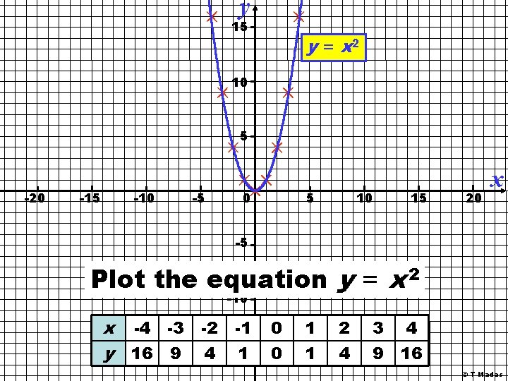
y 15 y = x 2 10 5 -20 -15 -10 -5 0 5 10 15 20 x -5 Plot the equation y = x 2 -10 x -4 -3 -2 -1 y 16 9 4 -15 1 0 0 1 1 2 4 3 4 9 16 © T Madas

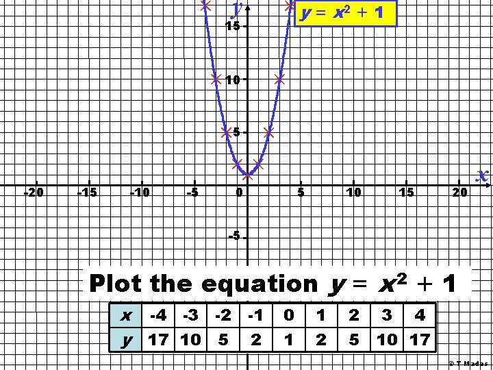
y y = x 2 + 1 15 10 5 -20 -15 -10 -5 0 5 10 15 20 x -5 2 + 1 Plot the equation y = x -10 x -4 -3 -2 -1 y 17 10 5 -15 2 0 1 1 2 2 3 4 5 10 17 © T Madas

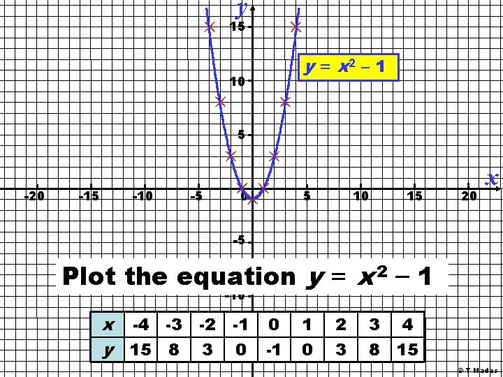
y 15 10 y = x 2 – 1 5 -20 -15 -10 -5 0 5 10 15 20 x -5 Plot the equation y = x 2 – 1 -10 x -4 -3 -2 -1 0 y 15 8 3 -15 0 -1 1 0 2 3 3 4 8 15 © T Madas

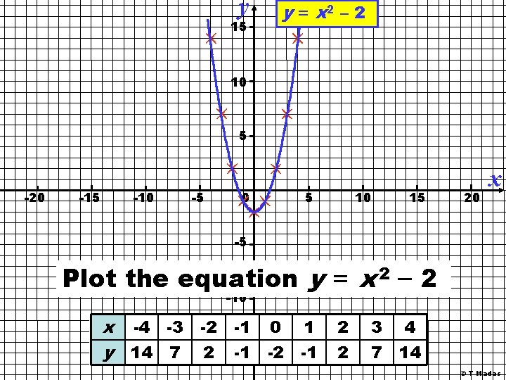
y 15 y = x 2 – 2 10 5 -20 -15 -10 -5 0 5 10 15 20 x -5 Plot the equation y = x 2 – 2 -10 x -4 -3 -2 -1 0 1 y 14 7 2 -15 -1 -2 -1 2 2 3 4 7 14 © T Madas

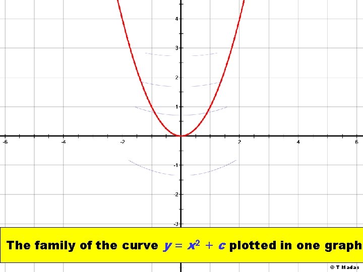
The family of the curve y = x 2 + c plotted in one graph © T Madas

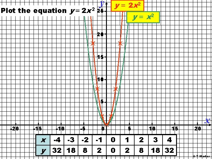
y Plot the equation y = 2 x 2 25 y = 2 x 2 y = x 2 20 15 10 5 -20 -15 -10 -5 0 x -4 -3 -2 -1 0 -5 y 32 18 8 2 0 5 1 2 10 15 2 3 4 8 18 32 20 x © T Madas

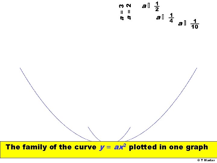
a=3 a=2 The family of the curve y = ax 2 plotted in one graph © T Madas

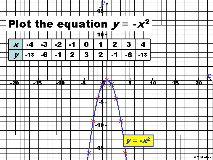
y 15 Plot the equation y = -x 2 10 x y -20 -4 -3 -2 -1 -13 -6 -1 2 -15 -10 0 3 -5 1 2 3 25 -1 -6 0 5 4 -13 10 15 20 x -5 -10 -15 y = -x 2 © T Madas

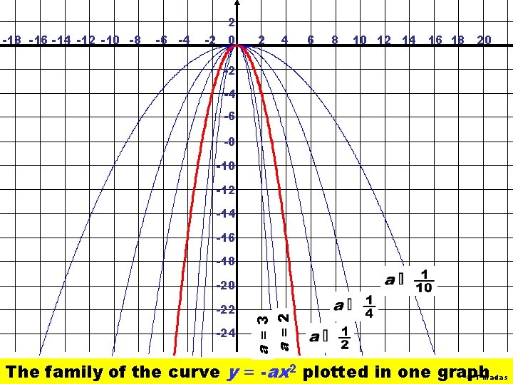
2 -18 -16 -14 -12 -10 -8 -6 -4 -2 0 2 4 6 8 10 12 14 16 18 20 -2 -4 -6 -8 -10 -12 -14 -16 -18 -22 -24 a=3 a=2 -20 The family of the curve y = -ax 2 plotted in one graph © T Madas

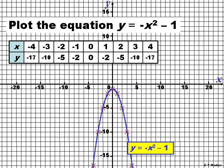
y 15 Plot the equation y = -x 2 – 1 10 x y -20 -4 -3 -2 -1 -17 -10 -5 -2 -15 -10 0 0 -5 1 2 -2 5 -5 0 3 4 -10 -17 5 10 15 20 x -5 -10 -15 y = -x 2 – 1 © T Madas

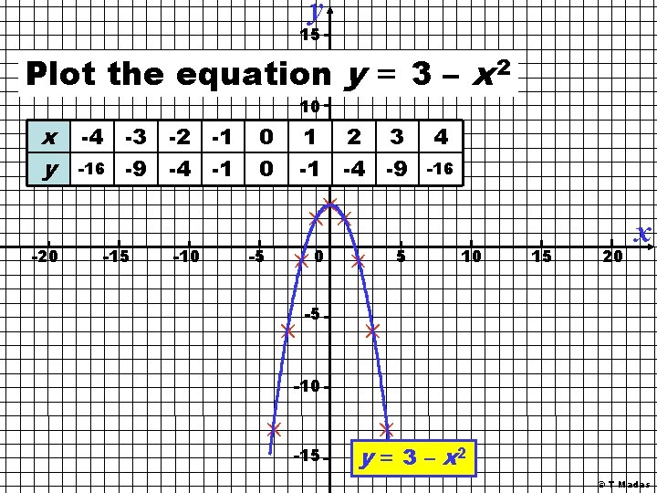
y 15 Plot the equation y = 3 – x 2 10 x y -20 -4 -3 -2 -1 -16 -9 -4 -1 -15 -10 0 0 -5 1 2 3 -1 5 -4 -9 0 5 4 -16 10 15 20 x -5 -10 -15 y = 3 – x 2 © T Madas

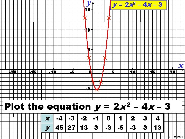
y 15 y = 2 x 2 – 4 x – 3 10 5 -20 -15 -10 -5 0 5 10 15 20 x -5 2 – 4 x – 3 Plot the equation y = 2 x -10 x -4 -3 -2 -1 0 1 2 y 45 27 13 -3 -5 -3 -15 3 3 4 3 13 © T Madas

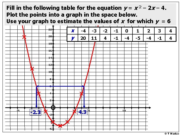
Fill in the following table for the equation y = x 2 – 2 x – 4. Plot the points into a graph in the space below. Use your graph 24 to estimate the values of x for which y = 6 22 20 x y -4 -3 -2 -1 0 1 2 3 4 20 11 4 -1 -4 -5 -4 -1 4 18 16 14 12 10 8 6 4 2 -5 -2. 3 -2 4. 3 5 10 -4 -6 © T Madas

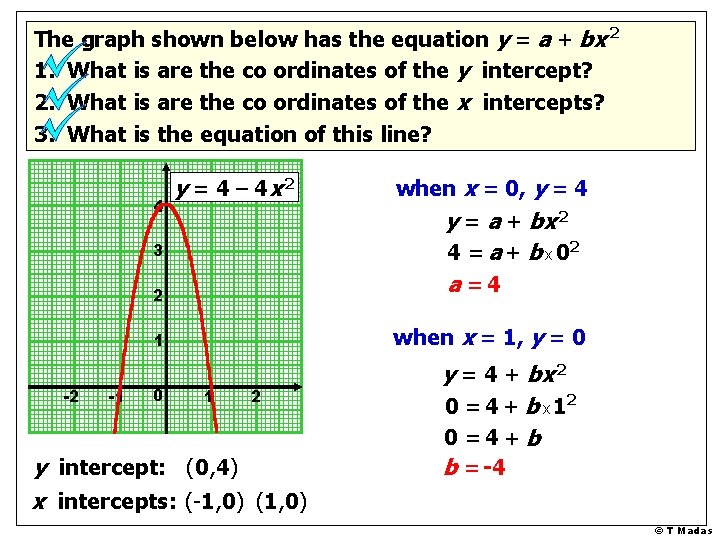
The graph shown below has the equation y = a + bx 2 1. What is are the co ordinates of the y intercept? 2. What is are the co ordinates of the x intercepts? 3. What is the equation of this line? 4 y = 4 – 4 x 2 3 2 when x = 1, y = 0 1 -2 -1 0 when x = 0, y = 4 y = a + bx 2 4 = a + b x 02 a =4 1 2 y intercept: (0, 4) x intercepts: (-1, 0) (1, 0) y = 4 + bx 2 0 = 4 + b x 12 0 =4+ b b = -4 © T Madas

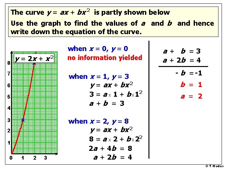
The curve y = ax + bx 2 is partly shown below Use the graph to find the values of a and b and hence write down the equation of the curve. 8 y = 2 x + x 2 7 when x = 1, y = 3 y = ax + bx 2 3 = a x 1 + b x 12 a +b = 3 6 5 4 3 2 1 0 when x = 0, y = 0 no information yielded 1 2 3 a + b =3 a + 2 b = 4 - b = -1 b = 1 a = 2 when x = 2, y = 8 y = ax + bx 2 8 = a x 2 + b x 22 2 a + 4 b = 8 a + 2 b = 4 © T Madas

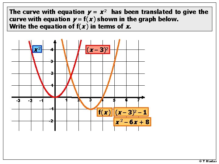
The curve with equation y = x 2 has been translated to give the curve with equation y = f(x ) shown in the graph below. Write the equation of f(x ) in terms of x. x 2 (x – 3)2 4 3 2 1 -3 -2 1 -1 -1 -2 2 3 4 5 6 7 f(x ) (x – 3)2 – 1 x 2 – 6 x + 8 © T Madas

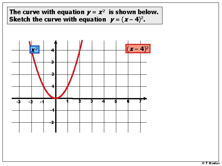
The curve with equation y = x 2 is shown below. Sketch the curve with equation y = (x – 4)2. x 2 (x – 4)2 4 3 2 1 -3 -2 1 -1 2 3 4 5 6 7 -1 -2 © T Madas

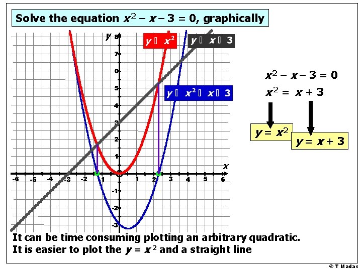
Solve the equation x 2 – x – 3 = 0, graphically y 8 7 6 x 2 – x – 3 = 0 x 2 = x + 3 5 4 3 y = x 2 2 1 -6 -5 -4 -3 -2 x 1 -1 y=x+3 2 3 4 5 6 -1 -2 -3 It can be time consuming plotting an arbitrary quadratic. It is easier to plot the y = x 2 and a straight line © T Madas

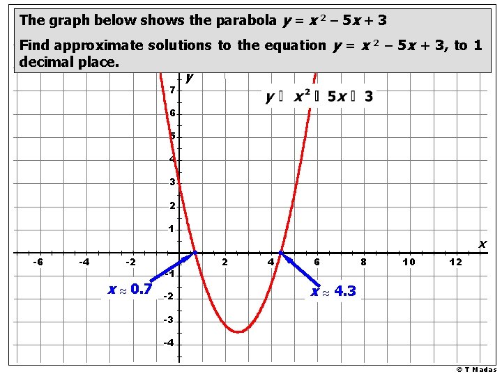
The graph below shows the parabola y = x 2 – 5 x + 3 Find approximate solutions to the equation y = x decimal place. 8 y 2 – 5 x + 3, to 1 7 6 5 4 3 2 1 -6 -4 -2 x ≈ 0. 7 -1 -2 x 2 4 6 8 10 12 x ≈ 4. 3 -3 -4 © T Madas

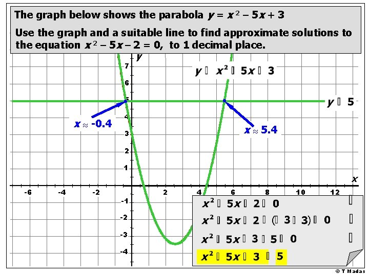
The graph below shows the parabola y = x 2 – 5 x + 3 Use the graph andsolutions a suitabletoline find approximate Find approximate thetoequation y = x 2 – solutions 5 x + 3, toto 1 the equation decimal place. x 2 – 5 x 8– 2 = 0, to 1 decimal place. y 7 6 5 x ≈ -0. 4 4 x ≈ 5. 4 3 2 1 -6 -4 -2 -1 x 2 4 6 8 10 12 -2 -3 -4 © T Madas