Quadratic Modeling 1 Quadratic Modeling WarmUp 2 Quadratic

Quadratic Modeling 1 Quadratic Modeling

Warm-Up 2 Quadratic Modeling

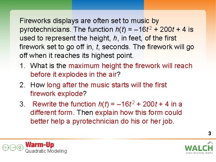
Fireworks displays are often set to music by pyrotechnicians. The function h(t) = – 16 t 2 + 200 t + 4 is used to represent the height, h, in feet, of the first firework set to go off in, t, seconds. The firework will go off when it reaches its highest point. 1. What is the maximum height the firework will reach before it explodes in the air? 2. How long after the music starts will the first firework explode? 3. Rewrite the function h(t) = – 16 t 2 + 200 t + 4 in a different form. Then explain how this form could better help a pyrotechnician do his or her job. 3 Quadratic Modeling

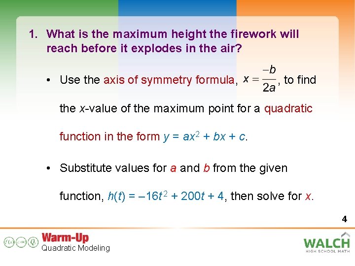
1. What is the maximum height the firework will reach before it explodes in the air? • Use the axis of symmetry formula, , to find the x-value of the maximum point for a quadratic function in the form y = ax 2 + bx + c. • Substitute values for a and b from the given function, h(t) = – 16 t 2 + 200 t + 4, then solve for x. 4 Quadratic Modeling

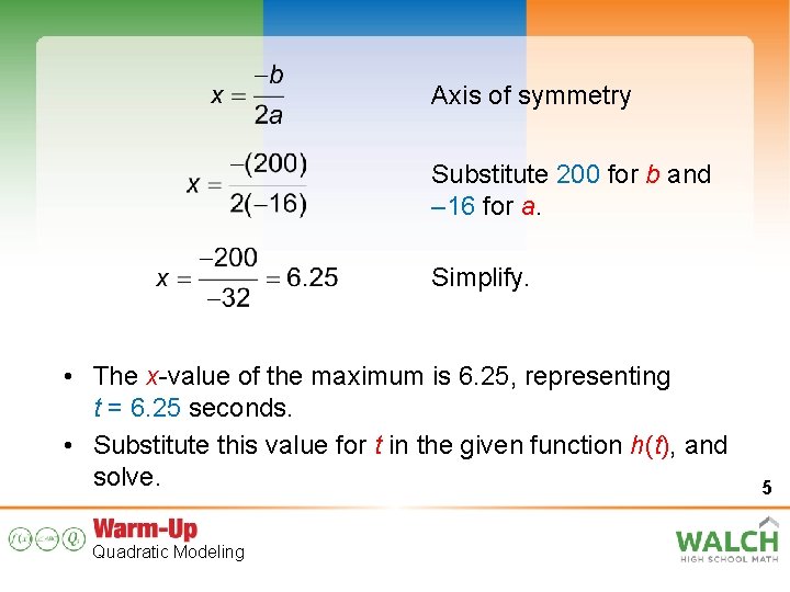
Axis of symmetry Substitute 200 for b and – 16 for a. Simplify. • The x-value of the maximum is 6. 25, representing t = 6. 25 seconds. • Substitute this value for t in the given function h(t), and solve. Quadratic Modeling 5

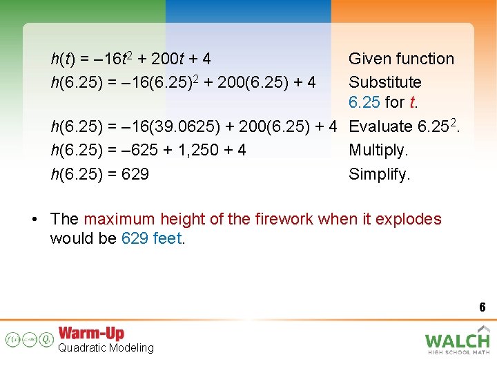
h(t) = – 16 t 2 + 200 t + 4 h(6. 25) = – 16(6. 25)2 + 200(6. 25) + 4 Given function Substitute 6. 25 for t. h(6. 25) = – 16(39. 0625) + 200(6. 25) + 4 Evaluate 6. 252. h(6. 25) = – 625 + 1, 250 + 4 Multiply. h(6. 25) = 629 Simplify. • The maximum height of the firework when it explodes would be 629 feet. 6 Quadratic Modeling

2. How long after the music starts will the first firework explode? • Using the maximum point that we found in problem 1, we know the firework will explode 6. 25 seconds after the music starts. 7 Quadratic Modeling

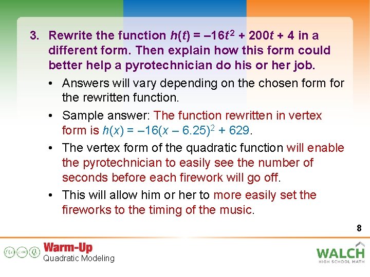
3. Rewrite the function h(t) = – 16 t 2 + 200 t + 4 in a different form. Then explain how this form could better help a pyrotechnician do his or her job. • Answers will vary depending on the chosen form for the rewritten function. • Sample answer: The function rewritten in vertex form is h(x) = – 16(x – 6. 25)2 + 629. • The vertex form of the quadratic function will enable the pyrotechnician to easily see the number of seconds before each firework will go off. • This will allow him or her to more easily set the fireworks to the timing of the music. 8 Quadratic Modeling

Instruction 9 Quadratic Modeling

Introduction • Even though we might not realize it, quadratic relationships are all around us. • When a basketball player shoots a three-pointer to win a game, the ball’s arc forms a parabola with a quadratic relationship relating the height of the ball to the time of its flight. 10 Quadratic Modeling

Introduction • When an architect is designing a room to use the least amount of materials to build a wall for a given area, the minimum perimeter is sometimes based on a quadratic relationship relating the area to the length and width of the room. • Being able to model, solve, and evaluate these equations can help us make predictions about the behavior of many real-world situations. 11 Quadratic Modeling

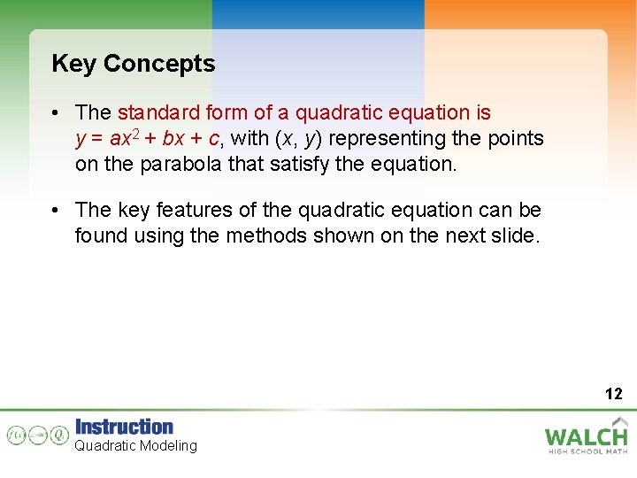
Key Concepts • The standard form of a quadratic equation is y = ax 2 + bx + c, with (x, y) representing the points on the parabola that satisfy the equation. • The key features of the quadratic equation can be found using the methods shown on the next slide. 12 Quadratic Modeling

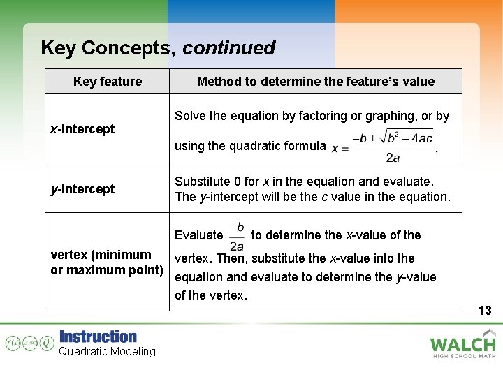
Key Concepts, continued Key feature x-intercept Method to determine the feature’s value Solve the equation by factoring or graphing, or by using the quadratic formula y-intercept Substitute 0 for x in the equation and evaluate. The y-intercept will be the c value in the equation. Evaluate to determine the x-value of the vertex (minimum vertex. Then, substitute the x-value into the or maximum point) equation and evaluate to determine the y-value of the vertex. 13 Quadratic Modeling

Key Concepts, continued • The key features can also be determined using a graphing calculator. • The y-intercept is shown as the c value in the equation, so it is not necessary to use the calculator to find it. 14 Quadratic Modeling

Key Concepts, continued • To find the x-intercepts: On a TI-83/84: Step 1: Press Y=, and type the quadratic equation in Y 1 and y = 0 in Y 2. Step 2: Adjust the calculator window as necessary so that the x-intercepts are visible in the graph window. (continued) Quadratic Modeling 15

Key Concepts, continued Step 3: Press [2 ND][TRACE][CALC], and scroll to 5: Intersect. Press ENTER to select the quadratic graph, then press ENTER again to select the horizontal line y = 0. Use the arrows to move the cursor near one of the x-intercepts. Press ENTER to find the intercept at (x, 0). The x-value represents the x-intercept. 16 Quadratic Modeling

Key Concepts, continued Step 4: If there is another x-intercept, press [2 ND][TRACE][CALC], and scroll to 5: Intersect. Press ENTER to select the quadratic graph, then press ENTER again to select the horizontal line y = 0. Use the arrows to move the cursor near the other x-intercept. Press ENTER to find the intercept at (x, 0). The x-value represents the second x-intercept. 17 Quadratic Modeling

Key Concepts, continued On a TI-Nspire: Step 1: Press the HOME key. Choose the Graphs and Geometry Application, then type the quadratic equation in f 1(x) and type f 2(x) = 0. Step 2: Adjust the viewing window so that all x-intercepts are visible on the graph. Step 3: Press MENU, select 6: Points & Lines, then select 3: Intersection Points. Step 4: When the pointing hand appears, click on the quadratic graph and line y = 0 (the x-axis). All xintercepts in the viewing window are displayed as (x, 0). The x-values are the x-intercepts. 18 Quadratic Modeling

Key Concepts, continued • To find the vertex on a TI-83/84: Step 1: Press Y=, and type the quadratic equation into Y 1. Step 2: Press WINDOW. Adjust the window range so that the vertex is visible on the graph. Step 3: Press GRAPH to see the graph. Then press [2 ND][TRACE][CALC] and scroll to #3 if the vertex is a minimum and #4 if the vertex is a maximum. Set the left bound anywhere to the left of the vertex and the right bound anywhere to the right of the vertex. Press ENTER again to find the vertex. Quadratic Modeling 19

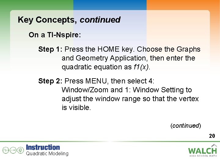
Key Concepts, continued On a TI-Nspire: Step 1: Press the HOME key. Choose the Graphs and Geometry Application, then enter the quadratic equation as f 1(x). Step 2: Press MENU, then select 4: Window/Zoom and 1: Window Setting to adjust the window range so that the vertex is visible. (continued) 20 Quadratic Modeling

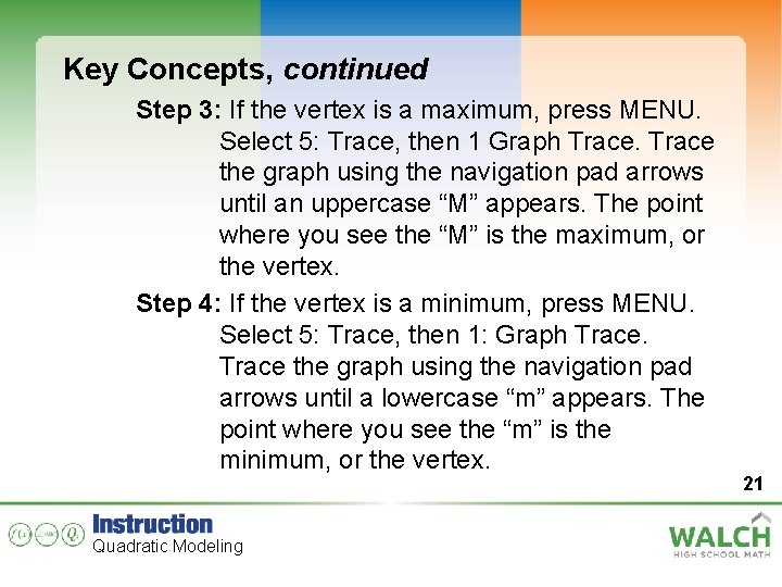
Key Concepts, continued Step 3: If the vertex is a maximum, press MENU. Select 5: Trace, then 1 Graph Trace the graph using the navigation pad arrows until an uppercase “M” appears. The point where you see the “M” is the maximum, or the vertex. Step 4: If the vertex is a minimum, press MENU. Select 5: Trace, then 1: Graph Trace the graph using the navigation pad arrows until a lowercase “m” appears. The point where you see the “m” is the minimum, or the vertex. Quadratic Modeling 21

Key Concepts, continued • When reading word problems in which you must use a quadratic equation to answer a question, certain keywords and phrases can help determine what key feature will help you answer the question. • The context of the problem is also extremely important, but the words and phrases on the next slide can be a guide: 22 Quadratic Modeling

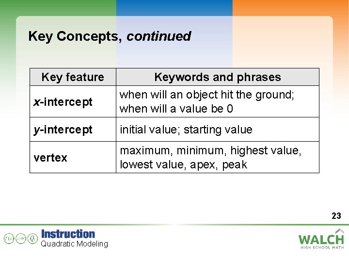
Key Concepts, continued Key feature x-intercept Keywords and phrases when will an object hit the ground; when will a value be 0 y-intercept initial value; starting value vertex maximum, minimum, highest value, lowest value, apex, peak 23 Quadratic Modeling

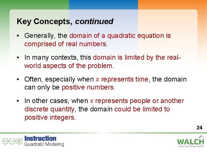
Key Concepts, continued • Generally, the domain of a quadratic equation is comprised of real numbers. • In many contexts, this domain is limited by the realworld aspects of the problem. • Often, especially when x represents time, the domain can only be positive numbers. • In other cases, when x represents people or another discrete quantity, the domain could be limited to positive integers. 24 Quadratic Modeling

Key Concepts, continued • It is important to consider the context of the problem when determining the potential answer to a word problem. • One common application of quadratic equations involves projectile motion, when objects are launched from a given height at a given velocity. • The rate at which they accelerate toward the ground due to gravity is represented by a quadratic equation. 25 Quadratic Modeling

Key Concepts, continued • For the standard form equation y = ax 2 + bx + c: • a will usually be – 4. 9 meters/second 2 or – 16 feet/second 2, representing the proven rate for gravity; • b will represent the initial velocity at which the object was launched; and • c will represent the initial height of the object. 26 Quadratic Modeling

Common Errors/Misconceptions • misinterpreting the question in a word problem and solving for the wrong feature • giving answers that are outside the domain of a given context, such as negative x-intercepts 27 Quadratic Modeling

Guided Practice Example 1 Given the quadratic function f(x) = – 2 x 2 + 8 x + 6, algebraically determine the axis of symmetry and the vertex. Identify whether the vertex represents a maximum or minimum. 28 Quadratic Modeling

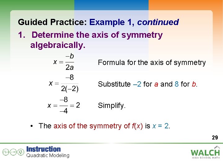
Guided Practice: Example 1, continued 1. Determine the axis of symmetry algebraically. Formula for the axis of symmetry Substitute – 2 for a and 8 for b. Simplify. • The axis of the symmetry of f(x) is x = 2. 29 Quadratic Modeling

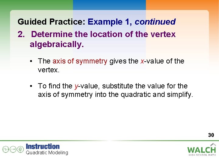
Guided Practice: Example 1, continued 2. Determine the location of the vertex algebraically. • The axis of symmetry gives the x-value of the vertex. • To find the y-value, substitute the value for the axis of symmetry into the quadratic and simplify. 30 Quadratic Modeling

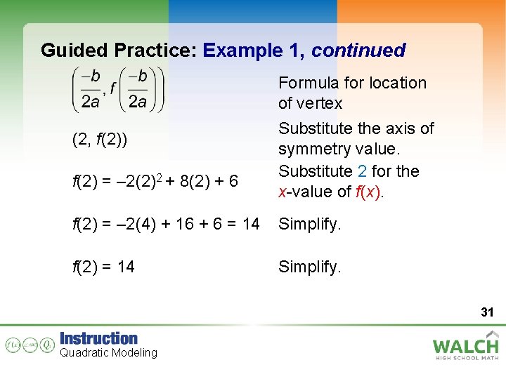
Guided Practice: Example 1, continued Formula for location of vertex (2, f(2)) f(2) = – 2(2)2 + 8(2) + 6 Substitute the axis of symmetry value. Substitute 2 for the x-value of f(x). f(2) = – 2(4) + 16 + 6 = 14 Simplify. f(2) = 14 Simplify. 31 Quadratic Modeling

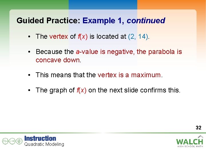
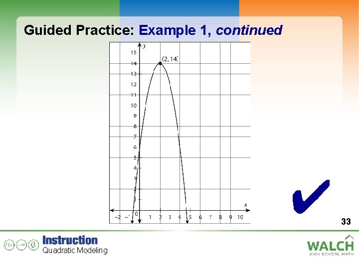
Guided Practice: Example 1, continued • The vertex of f(x) is located at (2, 14). • Because the a-value is negative, the parabola is concave down. • This means that the vertex is a maximum. • The graph of f(x) on the next slide confirms this. 32 Quadratic Modeling

Guided Practice: Example 1, continued ✔ Quadratic Modeling 33

Guided Practice: Example 1, continued 34 Quadratic Modeling

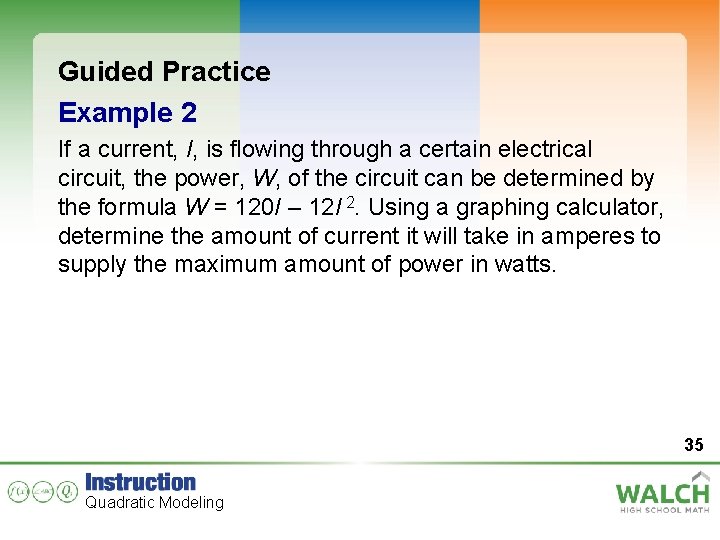
Guided Practice Example 2 If a current, I, is flowing through a certain electrical circuit, the power, W, of the circuit can be determined by the formula W = 120 I – 12 I 2. Using a graphing calculator, determine the amount of current it will take in amperes to supply the maximum amount of power in watts. 35 Quadratic Modeling

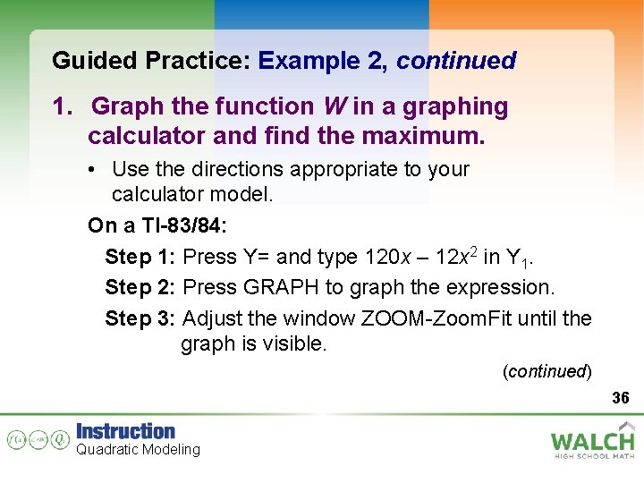
Guided Practice: Example 2, continued 1. Graph the function W in a graphing calculator and find the maximum. • Use the directions appropriate to your calculator model. On a TI-83/84: Step 1: Press Y= and type 120 x – 12 x 2 in Y 1. Step 2: Press GRAPH to graph the expression. Step 3: Adjust the window ZOOM-Zoom. Fit until the graph is visible. (continued) 36 Quadratic Modeling

Guided Practice: Example 2, continued Step 4: Press [2 ND][TRACE][CALC] and scroll to 4: Maximum. Set the left bound anywhere to the left of the vertex in the graph, and set the right bound anywhere to the right of the vertex in the graph to calculate the highest point. Press ENTER again to get point (4. 9999971300). 37 Quadratic Modeling

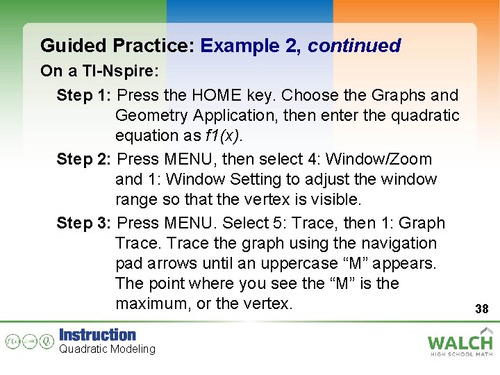
Guided Practice: Example 2, continued On a TI-Nspire: Step 1: Press the HOME key. Choose the Graphs and Geometry Application, then enter the quadratic equation as f 1(x). Step 2: Press MENU, then select 4: Window/Zoom and 1: Window Setting to adjust the window range so that the vertex is visible. Step 3: Press MENU. Select 5: Trace, then 1: Graph Trace the graph using the navigation pad arrows until an uppercase “M” appears. The point where you see the “M” is the maximum, or the vertex. Quadratic Modeling 38

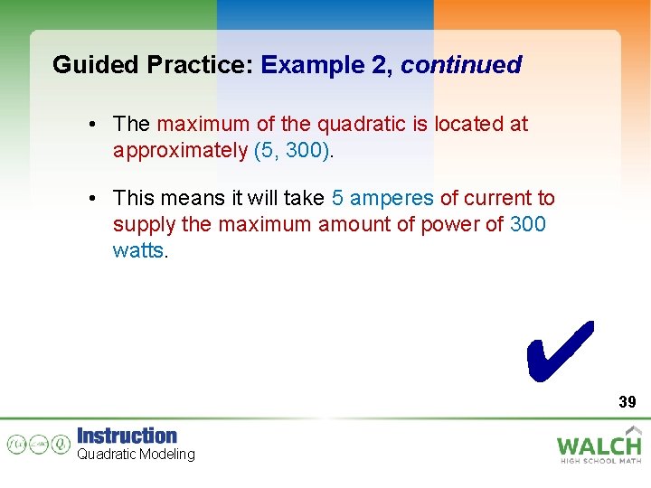
Guided Practice: Example 2, continued • The maximum of the quadratic is located at approximately (5, 300). • This means it will take 5 amperes of current to supply the maximum amount of power of 300 watts. ✔ Quadratic Modeling 39

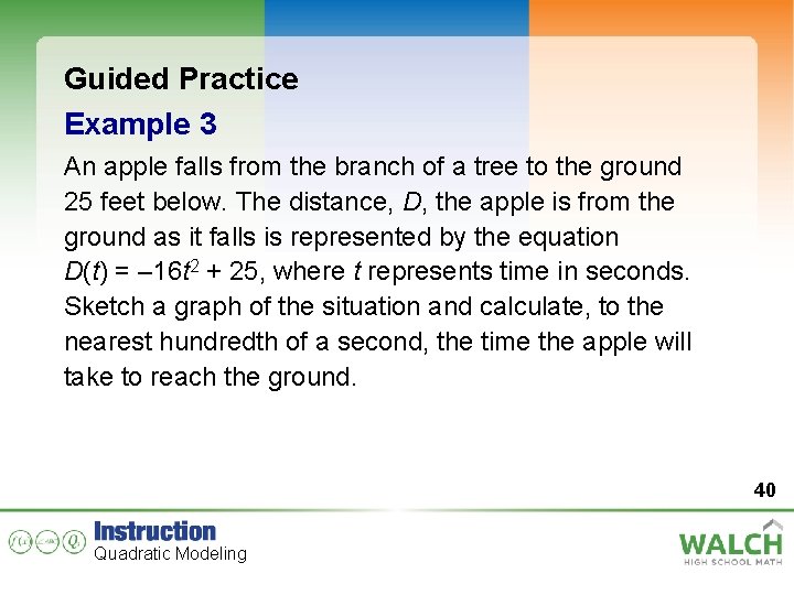
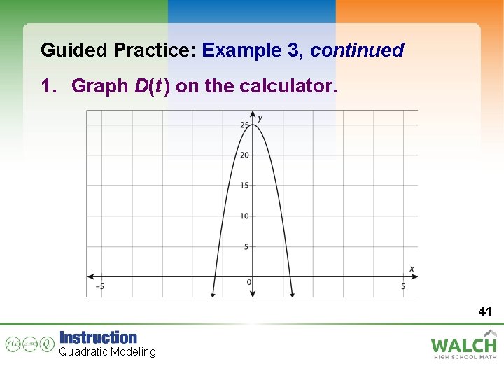
Guided Practice Example 3 An apple falls from the branch of a tree to the ground 25 feet below. The distance, D, the apple is from the ground as it falls is represented by the equation D(t) = – 16 t 2 + 25, where t represents time in seconds. Sketch a graph of the situation and calculate, to the nearest hundredth of a second, the time the apple will take to reach the ground. 40 Quadratic Modeling

Guided Practice: Example 3, continued 1. Graph D(t ) on the calculator. 41 Quadratic Modeling

Guided Practice: Example 3, continued 2. Algebraically determine the time it will take the apple to reach the ground. • The time it takes the apple to reach the ground represents the x-intercept of D(t). • When the apple is on the ground, D(t), or the distance the apple is from the ground, equals 0. • Solve for the x-intercept by replacing D(t) with 0. 42 Quadratic Modeling

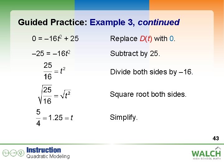
Guided Practice: Example 3, continued 0 = – 16 t 2 + 25 Replace D(t) with 0. – 25 = – 16 t 2 Subtract by 25. Divide both sides by – 16. Square root both sides. Simplify. 43 Quadratic Modeling

Guided Practice: Example 3, continued 3. Confirm the x-intercept found in the previous step using the graphing calculator. On a TI-83/84: Step 1: Press Y=, and type the quadratic equation in Y 1 and y = 0 in Y 2. Step 2: Adjust the calculator window as necessary so that the x-intercepts are visible in the graph window. 44 Quadratic Modeling

Guided Practice: Example 3, continued Step 3: Press [2 ND][TRACE][CALC] and scroll to 5: Intersect. Press [ENTER] to select the quadratic graph, then press [ENTER] again to select the horizontal line y = 0. Use the arrows to move the cursor near the right xintercept. Press [ENTER] to find the intercept at (x, 0). 45 Quadratic Modeling

Guided Practice: Example 3, continued On a TI-Nspire: Step 1: From the Graphs and Geometry Application, type the quadratic equation in f 1(x) and type f 2(x) = 0. Step 2: Adjust the viewing window so that all xintercepts are visible on the graph. Step 3: Press [menu] and select 6: Points & Lines, then 3: Intersection Points. Step 4: When the pointing hand appears, click on the quadratic graph. The line y = 0 (the xaxis) and all x-intercepts in the viewing window will be displayed as (x, 0). Quadratic Modeling 46

Guided Practice: Example 3, continued • The x-value of (1. 25, 0) represents the positive x-intercept. • It will take the apple 1. 25 seconds to reach the ground. ✔ Quadratic Modeling 47

Guided Practice: Example 3, continued 48 Quadratic Modeling

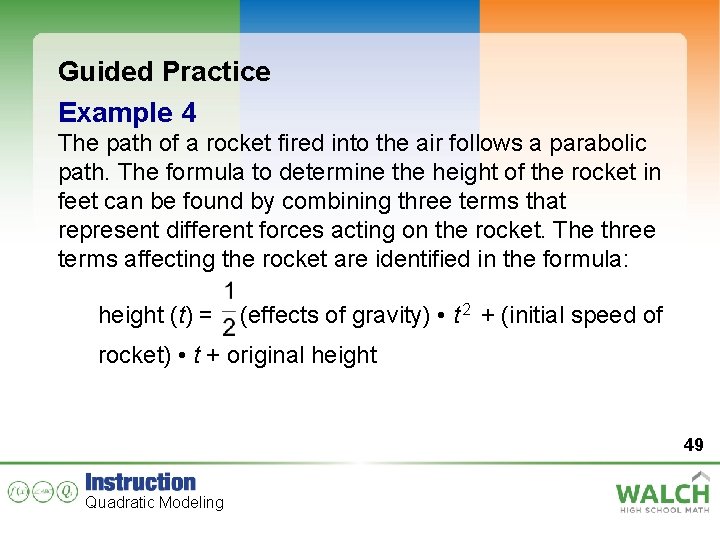
Guided Practice Example 4 The path of a rocket fired into the air follows a parabolic path. The formula to determine the height of the rocket in feet can be found by combining three terms that represent different forces acting on the rocket. The three terms affecting the rocket are identified in the formula: height (t) = (effects of gravity) • t 2 + (initial speed of rocket) • t + original height 49 Quadratic Modeling

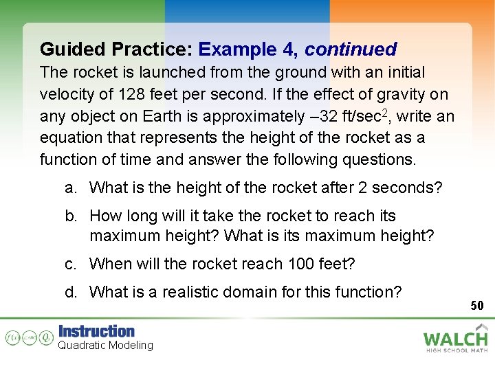
Guided Practice: Example 4, continued The rocket is launched from the ground with an initial velocity of 128 feet per second. If the effect of gravity on any object on Earth is approximately – 32 ft/sec 2, write an equation that represents the height of the rocket as a function of time and answer the following questions. a. What is the height of the rocket after 2 seconds? b. How long will it take the rocket to reach its maximum height? What is its maximum height? c. When will the rocket reach 100 feet? d. What is a realistic domain for this function? Quadratic Modeling 50

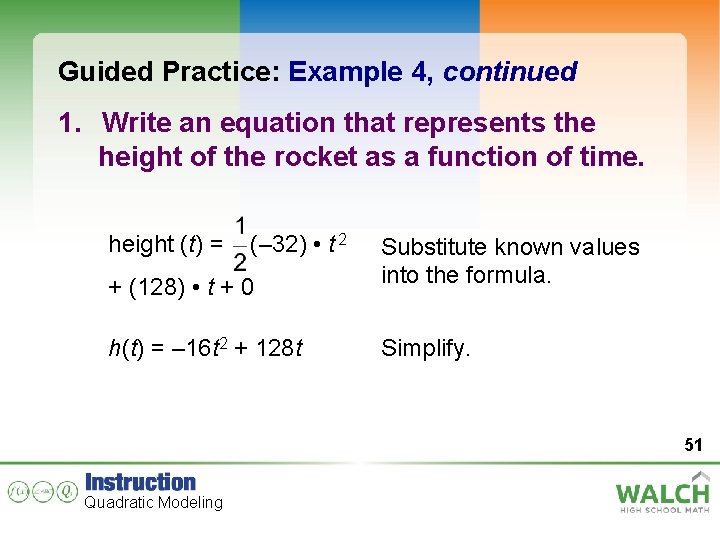
Guided Practice: Example 4, continued 1. Write an equation that represents the height of the rocket as a function of time. height (t) = (– 32) • t 2 + (128) • t + 0 Substitute known values into the formula. h(t) = – 16 t 2 + 128 t Simplify. 51 Quadratic Modeling

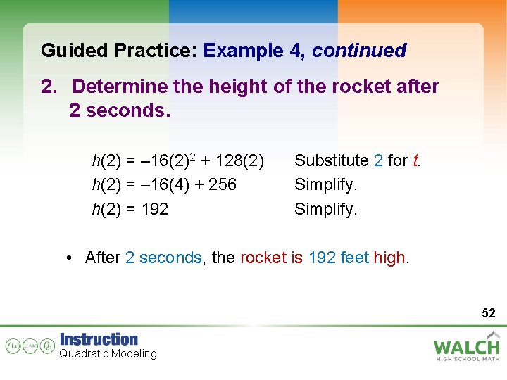
Guided Practice: Example 4, continued 2. Determine the height of the rocket after 2 seconds. h(2) = – 16(2)2 + 128(2) h(2) = – 16(4) + 256 h(2) = 192 Substitute 2 for t. Simplify. • After 2 seconds, the rocket is 192 feet high. 52 Quadratic Modeling

Guided Practice: Example 4, continued 3. Determine the location of the maximum using a graphing calculator. On a TI-83/84: Step 1: Press Y= and type – 16 x 2 + 128 x in Y 1. Step 2: Press GRAPH to graph the expression. Step 3: Adjust the window ZOOM-Zoom. Fit until the graph is visible. (continued) Quadratic Modeling 53

Guided Practice: Example 4, continued Step 4: Press [2 ND][TRACE][CALC] and scroll to 4: Maximum. Set the left bound anywhere to the left of the vertex in the graph, and set the right bound anywhere to the right of the vertex in the graph to calculate the highest point. Press [ENTER] again to get point (3. 9999981256). 54 Quadratic Modeling

Guided Practice: Example 4, continued On a TI-Nspire: Step 1: Press the HOME key. Choose the Graphs and Geometry Application, then enter the quadratic equation as f 1(x). Step 2: Press MENU, then select 4: Window/Zoom and 1: Window Setting to adjust the window range so that the vertex is visible. Step 3: Press MENU. Select 5: Trace, then 1: Graph Trace the graph using the navigation pad arrows until an uppercase “M” appears. The point where you see the “M” is the maximum, or the vertex. Quadratic Modeling 55

Guided Practice: Example 4, continued • The maximum of the quadratic function is approximately (4, 256). • It will take the rocket 4 seconds to reach its maximum height of 256 feet in the air. 56 Quadratic Modeling

Guided Practice: Example 4, continued 4. Use the graphing calculator to determine when the rocket will reach 100 feet. On a TI-83/84: Step 1: Press Y=, and type the quadratic equation in Y 1 and y = 100 in Y 2. Step 2: Press GRAPH to graph both expressions on the same coordinate plane. Step 3: Adjust the window ZOOM-Zoom. Fit until the point of intersection is visible. (continued) Quadratic Modeling 57

Guided Practice: Example 4, continued Step 4: Press [2 ND][TRACE][CALC] and scroll to 5: Intersect. Press [ENTER] to select the first graph, then press [ENTER] again to select the second graph. Press [ENTER] to find the left point of intersection. The left point of intersection is at x = 0. 8775, y = 100. (continued) Quadratic Modeling 58

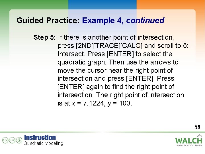
Guided Practice: Example 4, continued Step 5: If there is another point of intersection, press [2 ND][TRACE][CALC] and scroll to 5: Intersect. Press [ENTER] to select the quadratic graph. Then use the arrows to move the cursor near the right point of intersection and press [ENTER]. Press [ENTER] again to find the right point of intersection. The right point of intersection is at x = 7. 1224, y = 100. 59 Quadratic Modeling

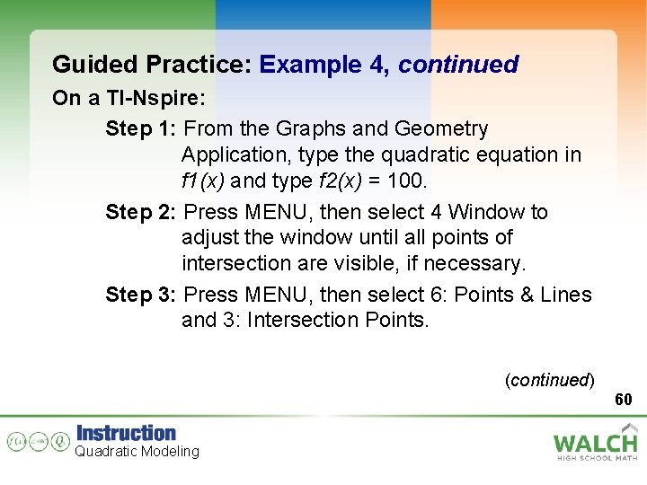
Guided Practice: Example 4, continued On a TI-Nspire: Step 1: From the Graphs and Geometry Application, type the quadratic equation in f 1(x) and type f 2(x) = 100. Step 2: Press MENU, then select 4 Window to adjust the window until all points of intersection are visible, if necessary. Step 3: Press MENU, then select 6: Points & Lines and 3: Intersection Points. (continued) 60 Quadratic Modeling

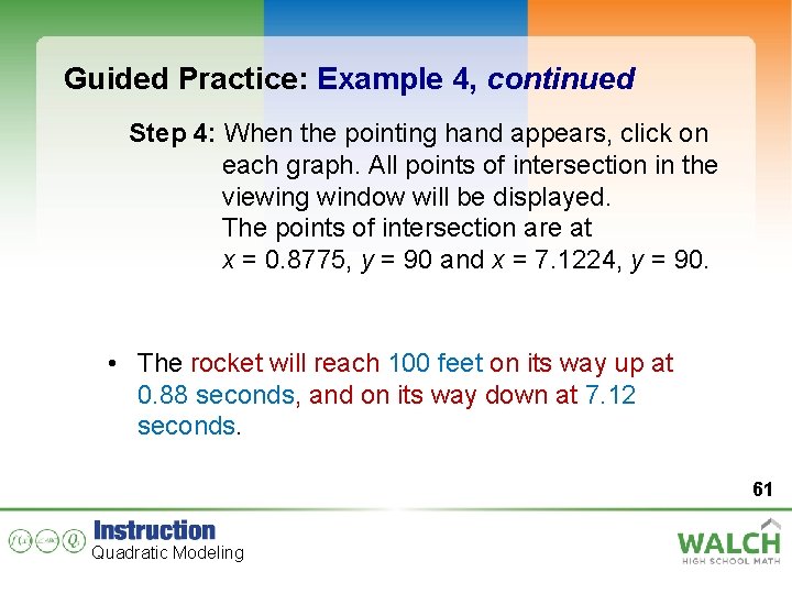
Guided Practice: Example 4, continued Step 4: When the pointing hand appears, click on each graph. All points of intersection in the viewing window will be displayed. The points of intersection are at x = 0. 8775, y = 90 and x = 7. 1224, y = 90. • The rocket will reach 100 feet on its way up at 0. 88 seconds, and on its way down at 7. 12 seconds. 61 Quadratic Modeling

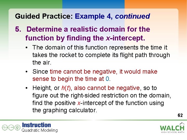
Guided Practice: Example 4, continued 5. Determine a realistic domain for the function by finding the x-intercept. • The domain of this function represents the time it takes the rocket to complete its flight path through the air. • Since time cannot be negative, it would make sense to begin the time at 0. • Height, or h(t), also cannot be negative, so to figure out the right-sided restriction on the domain, find the positive x-intercept of the function using the graphing calculator. Quadratic Modeling 62

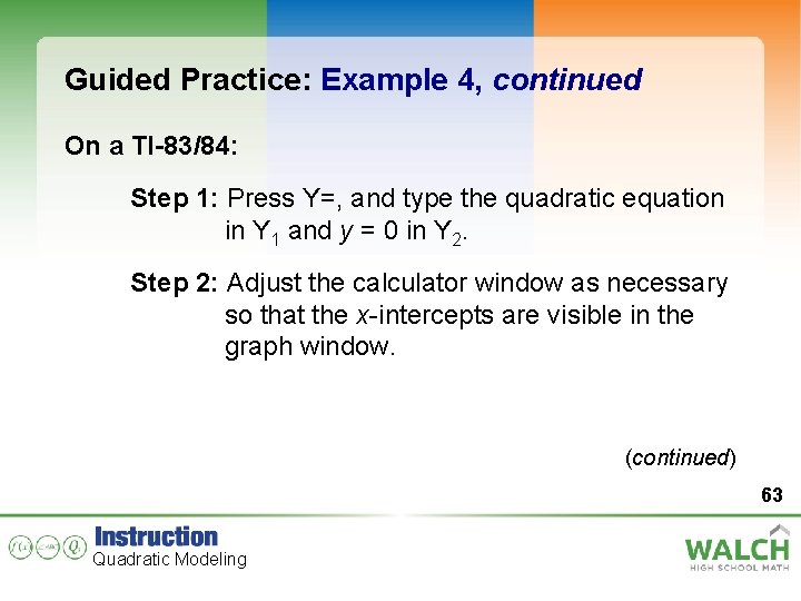
Guided Practice: Example 4, continued On a TI-83/84: Step 1: Press Y=, and type the quadratic equation in Y 1 and y = 0 in Y 2. Step 2: Adjust the calculator window as necessary so that the x-intercepts are visible in the graph window. (continued) 63 Quadratic Modeling

Guided Practice: Example 4, continued Step 3: Press [2 ND][TRACE][CALC] and scroll to 5: Intersect. Press [ENTER] to select the quadratic graph, then press [ENTER] again to select the horizontal line y = 0. Use the arrows to move the cursor near the right x-intercept. Press [ENTER] to find the intercept at (x, 0). The x-value of (8, 0) represents the positive x-intercept. 64 Quadratic Modeling

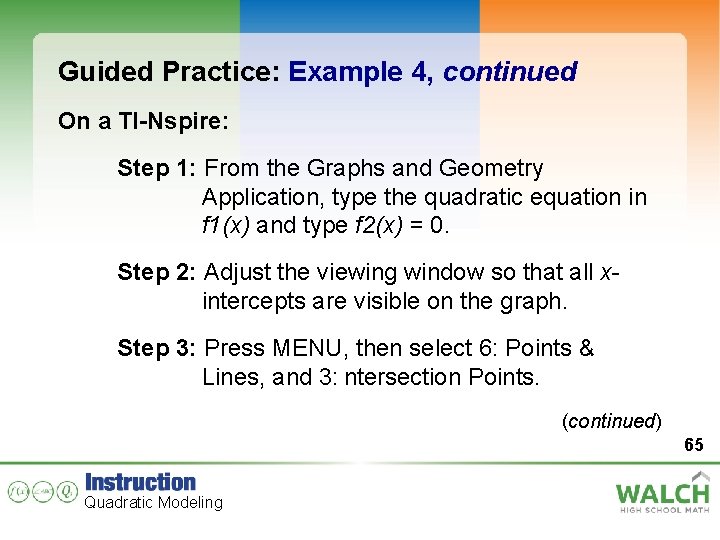
Guided Practice: Example 4, continued On a TI-Nspire: Step 1: From the Graphs and Geometry Application, type the quadratic equation in f 1(x) and type f 2(x) = 0. Step 2: Adjust the viewing window so that all xintercepts are visible on the graph. Step 3: Press MENU, then select 6: Points & Lines, and 3: ntersection Points. (continued) 65 Quadratic Modeling

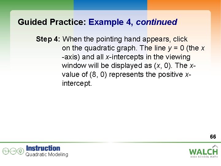
Guided Practice: Example 4, continued Step 4: When the pointing hand appears, click on the quadratic graph. The line y = 0 (the x -axis) and all x-intercepts in the viewing window will be displayed as (x, 0). The xvalue of (8, 0) represents the positive xintercept. 66 Quadratic Modeling

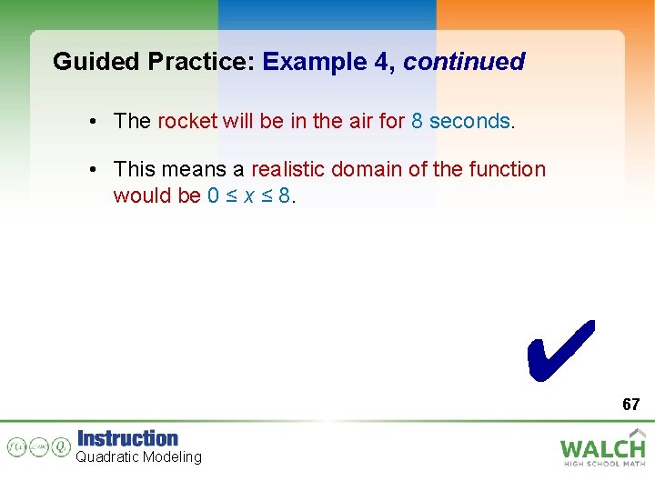
Guided Practice: Example 4, continued • The rocket will be in the air for 8 seconds. • This means a realistic domain of the function would be 0 ≤ x ≤ 8. ✔ 67 Quadratic Modeling