MSCIT 5210 Knowledge Discovery and Data Mining Acknowledgement

MSCIT 5210: Knowledge Discovery and Data Mining Acknowledgement: Slides modified by Dr. Lei Chen based on the slides provided by Jiawei Han, Micheline Kamber, and Jian Pei and Raymond Wong © 2012 Han, Kamber & Pei &Wong All rights reserved. 1 1

Outline of Advanced Clustering Analysis n Probability Model-Based Clustering n n Each object may take a probability to belong to a cluster Clustering High-Dimensional Data n Curse of dimensionality: Difficulty of distance measure in high-D space 2

Chapter 11. Cluster Analysis: Advanced Methods n Probability Model-Based Clustering n Clustering High-Dimensional Data n Summary 3

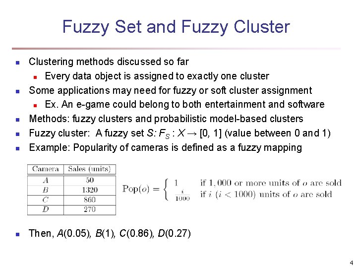
Fuzzy Set and Fuzzy Cluster n Clustering methods discussed so far n Every data object is assigned to exactly one cluster Some applications may need for fuzzy or soft cluster assignment n Ex. An e-game could belong to both entertainment and software Methods: fuzzy clusters and probabilistic model-based clusters Fuzzy cluster: A fuzzy set S: FS : X → [0, 1] (value between 0 and 1) Example: Popularity of cameras is defined as a fuzzy mapping n Then, A(0. 05), B(1), C(0. 86), D(0. 27) n n 4

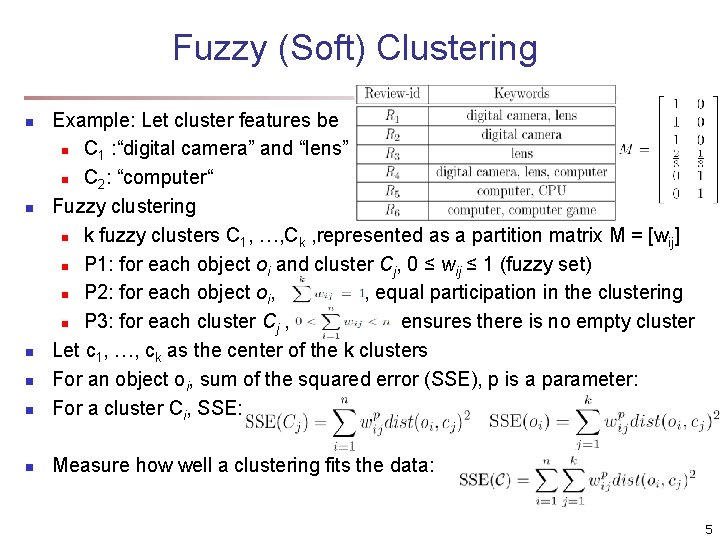
Fuzzy (Soft) Clustering n Example: Let cluster features be n C 1 : “digital camera” and “lens” n C 2: “computer“ Fuzzy clustering n k fuzzy clusters C 1, …, Ck , represented as a partition matrix M = [wij] n P 1: for each object oi and cluster Cj, 0 ≤ wij ≤ 1 (fuzzy set) n P 2: for each object oi, , equal participation in the clustering n P 3: for each cluster Cj , ensures there is no empty cluster Let c 1, …, ck as the center of the k clusters For an object oi, sum of the squared error (SSE), p is a parameter: For a cluster Ci, SSE: n Measure how well a clustering fits the data: n n 5

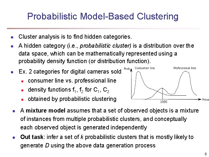
Probabilistic Model-Based Clustering n n n Cluster analysis is to find hidden categories. A hidden category (i. e. , probabilistic cluster) is a distribution over the data space, which can be mathematically represented using a probability density function (or distribution function). Ex. 2 categories for digital cameras sold n consumer line vs. professional line n density functions f 1, f 2 for C 1, C 2 n obtained by probabilistic clustering A mixture model assumes that a set of observed objects is a mixture of instances from multiple probabilistic clusters, and conceptually each observed object is generated independently Out task: infer a set of k probabilistic clusters that is mostly likely to generate D using the above data generation process 6

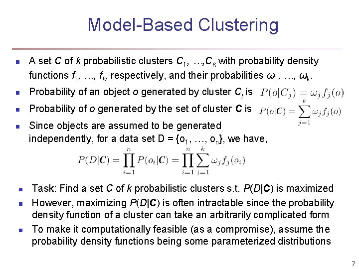
Model-Based Clustering n A set C of k probabilistic clusters C 1, …, Ck with probability density functions f 1, …, fk, respectively, and their probabilities ω1, …, ωk. n Probability of an object o generated by cluster Cj is n Probability of o generated by the set of cluster C is n n Since objects are assumed to be generated independently, for a data set D = {o 1, …, on}, we have, Task: Find a set C of k probabilistic clusters s. t. P(D|C) is maximized However, maximizing P(D|C) is often intractable since the probability density function of a cluster can take an arbitrarily complicated form To make it computationally feasible (as a compromise), assume the probability density functions being some parameterized distributions 7

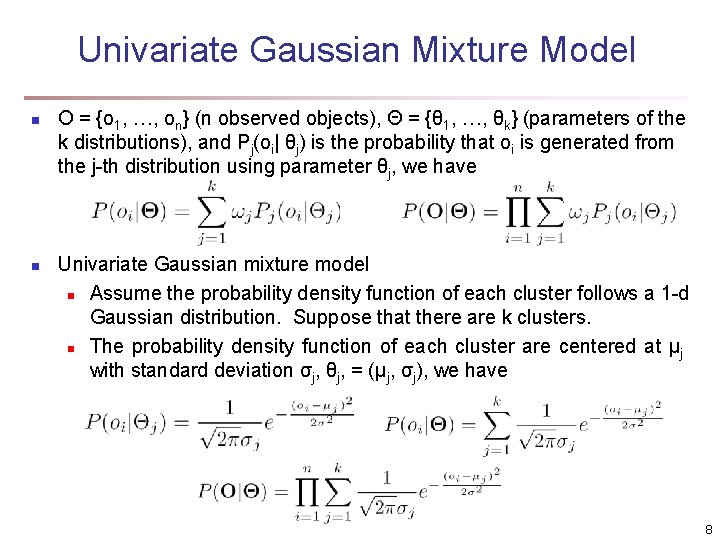
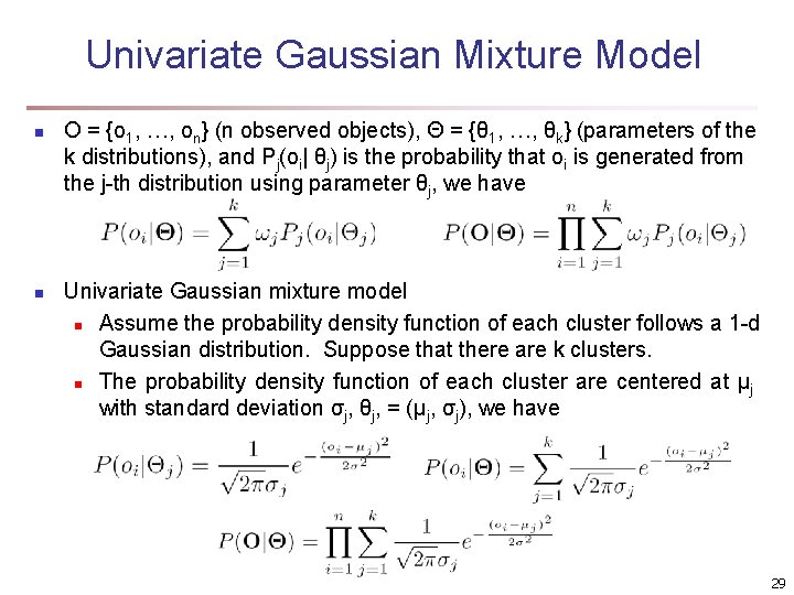
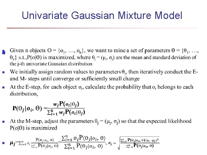
Univariate Gaussian Mixture Model n n O = {o 1, …, on} (n observed objects), Θ = {θ 1, …, θk} (parameters of the k distributions), and Pj(oi| θj) is the probability that oi is generated from the j-th distribution using parameter θj, we have Univariate Gaussian mixture model n Assume the probability density function of each cluster follows a 1 -d Gaussian distribution. Suppose that there are k clusters. n The probability density function of each cluster are centered at μj with standard deviation σj, θj, = (μj, σj), we have 8

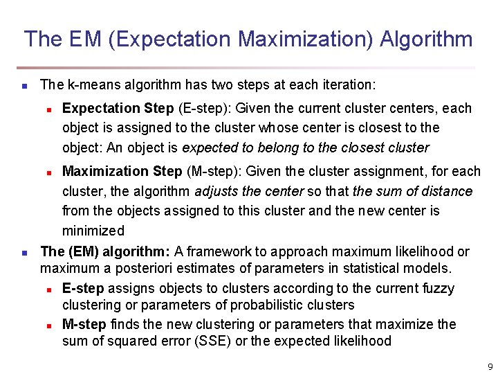
The EM (Expectation Maximization) Algorithm n The k-means algorithm has two steps at each iteration: n Expectation Step (E-step): Given the current cluster centers, each object is assigned to the cluster whose center is closest to the object: An object is expected to belong to the closest cluster Maximization Step (M-step): Given the cluster assignment, for each cluster, the algorithm adjusts the center so that the sum of distance from the objects assigned to this cluster and the new center is minimized The (EM) algorithm: A framework to approach maximum likelihood or maximum a posteriori estimates of parameters in statistical models. n E-step assigns objects to clusters according to the current fuzzy clustering or parameters of probabilistic clusters n M-step finds the new clustering or parameters that maximize the sum of squared error (SSE) or the expected likelihood n n 9

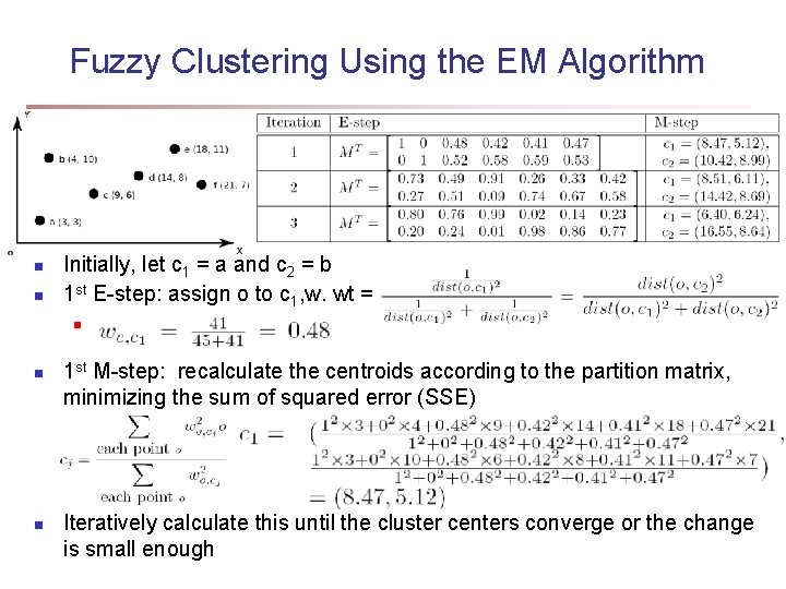
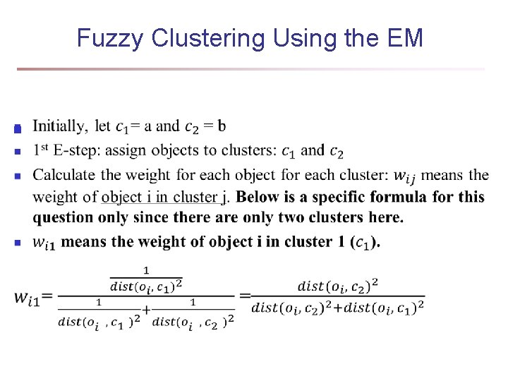
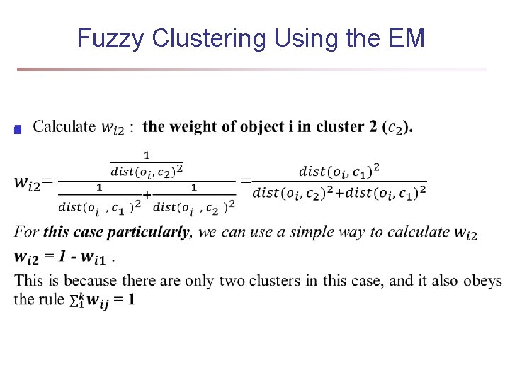
Fuzzy Clustering Using the EM Algorithm n n Initially, let c 1 = a and c 2 = b 1 st E-step: assign o to c 1, w. wt = n 1 st M-step: recalculate the centroids according to the partition matrix, minimizing the sum of squared error (SSE) Iteratively calculate this until the cluster centers converge or the change is small enough

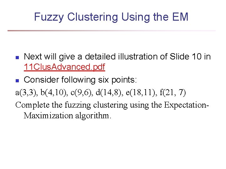
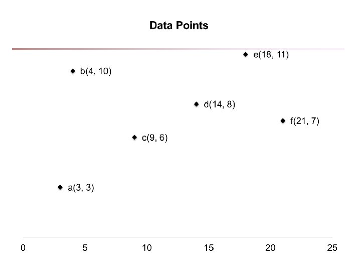
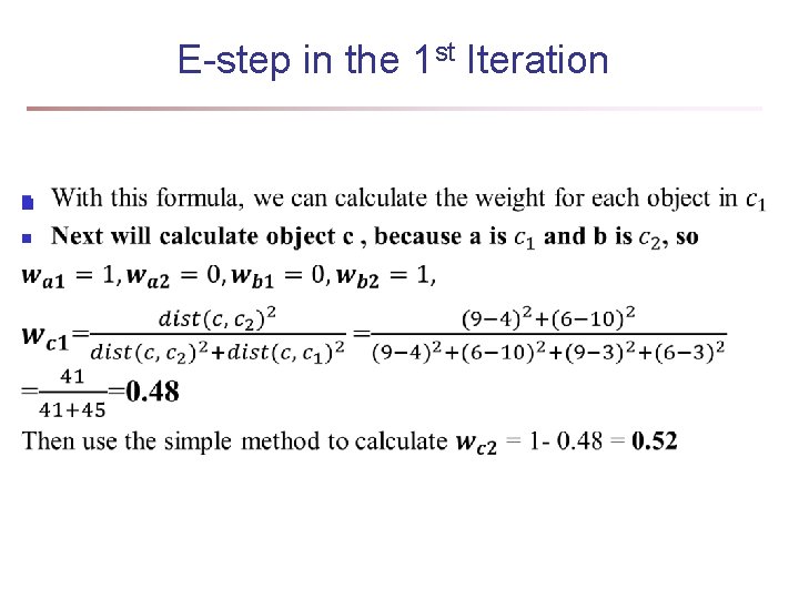
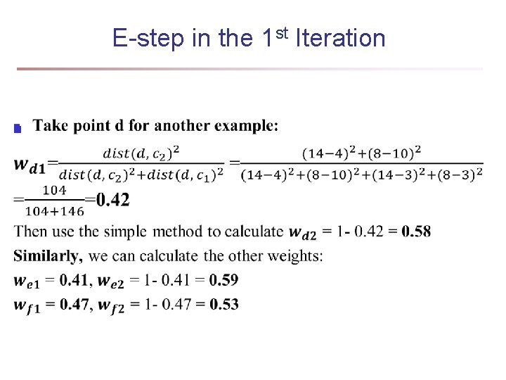
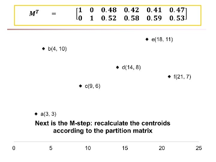
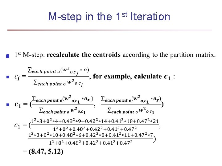
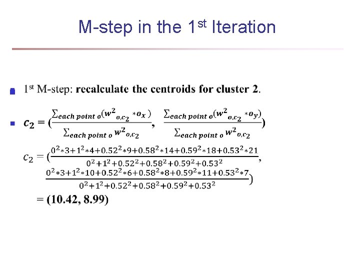
Fuzzy Clustering Using the EM Next will give a detailed illustration of Slide 10 in 11 Clus. Advanced. pdf n Consider following six points: a(3, 3), b(4, 10), c(9, 6), d(14, 8), e(18, 11), f(21, 7) Complete the fuzzing clustering using the Expectation. Maximization algorithm. n

Fuzzy Clustering Using the EM n

Fuzzy Clustering Using the EM n

E-step in the 1 st Iteration n

E-step in the 1 st Iteration n

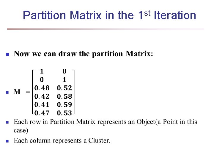
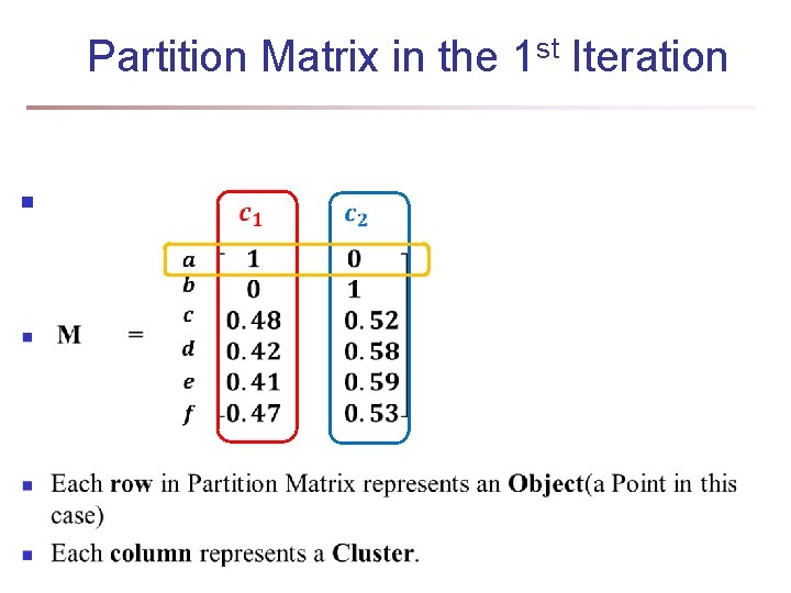
Partition Matrix in the 1 st Iteration n

Partition Matrix in the 1 st Iteration n

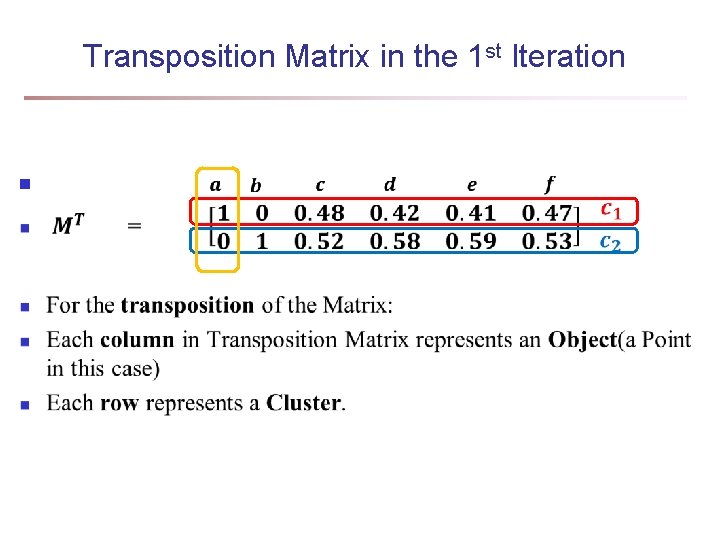
Transposition Matrix in the 1 st Iteration n

M-step in the 1 st Iteration n

M-step in the 1 st Iteration n

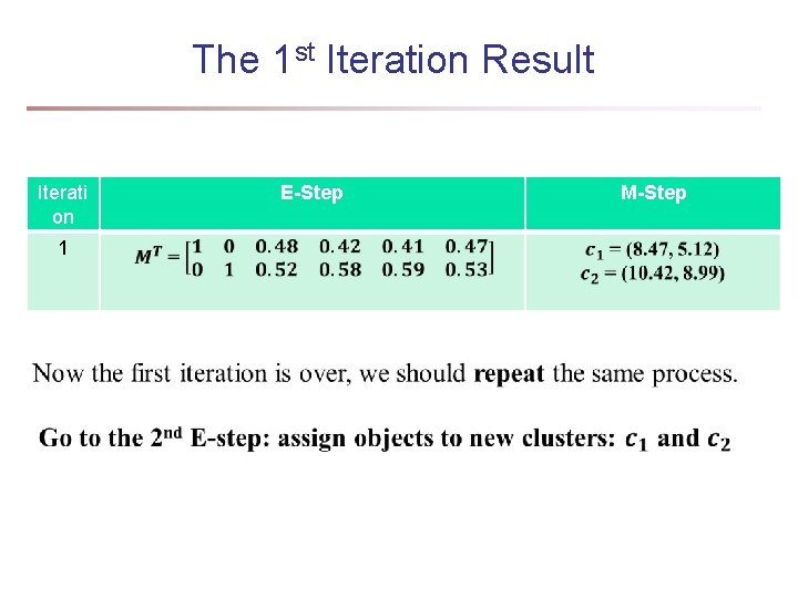
The 1 st Iteration Result Iterati on 1 E-Step M-Step

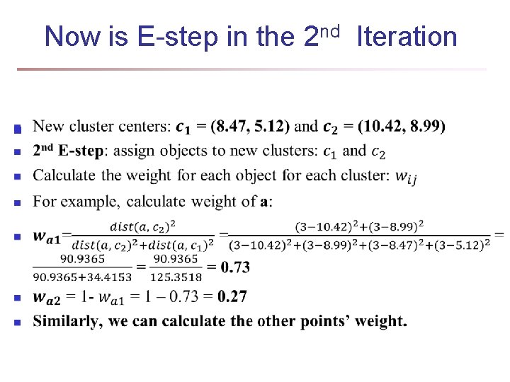
Now is E-step in the 2 nd Iteration n

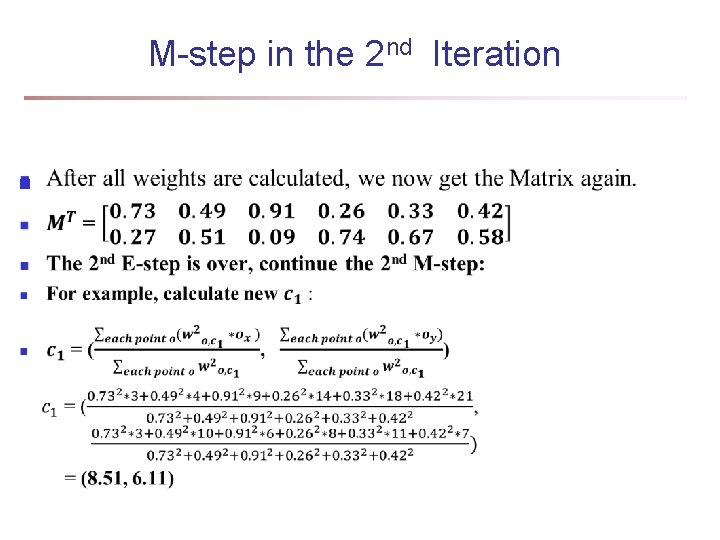
M-step in the 2 nd Iteration n

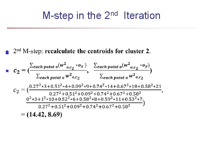
M-step in the 2 nd Iteration n

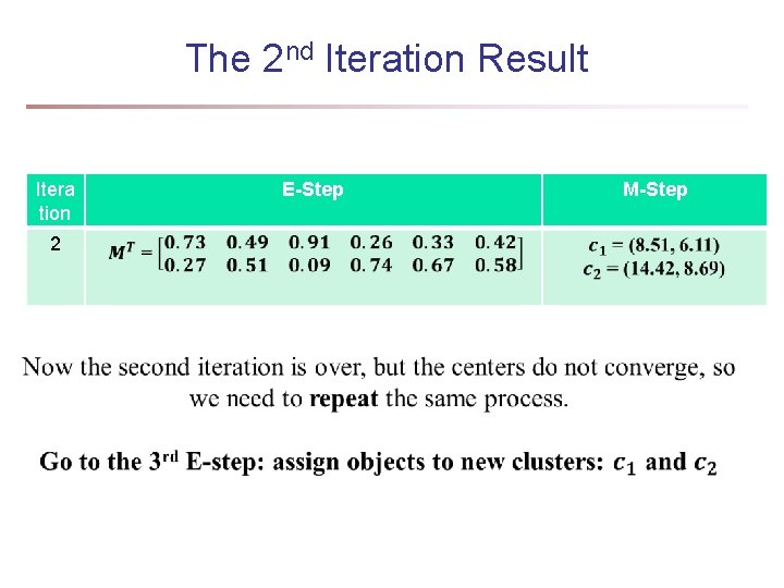
The 2 nd Iteration Result Itera tion 2 E-Step M-Step

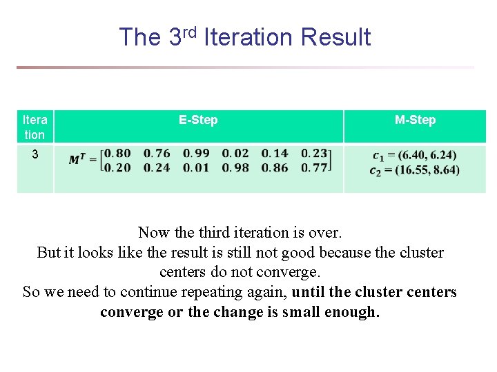
The 3 rd Iteration Result Itera tion E-Step M-Step 3 Now the third iteration is over. But it looks like the result is still not good because the cluster centers do not converge. So we need to continue repeating again, until the cluster centers converge or the change is small enough.

Univariate Gaussian Mixture Model n n O = {o 1, …, on} (n observed objects), Θ = {θ 1, …, θk} (parameters of the k distributions), and Pj(oi| θj) is the probability that oi is generated from the j-th distribution using parameter θj, we have Univariate Gaussian mixture model n Assume the probability density function of each cluster follows a 1 -d Gaussian distribution. Suppose that there are k clusters. n The probability density function of each cluster are centered at μj with standard deviation σj, θj, = (μj, σj), we have 29

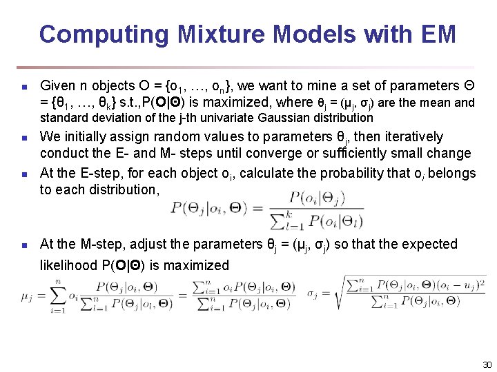
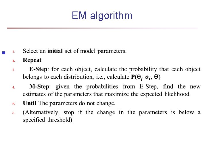
Computing Mixture Models with EM n Given n objects O = {o 1, …, on}, we want to mine a set of parameters Θ = {θ 1, …, θk} s. t. , P(O|Θ) is maximized, where θj = (μj, σj) are the mean and standard deviation of the j-th univariate Gaussian distribution n n n We initially assign random values to parameters θj, then iteratively conduct the E- and M- steps until converge or sufficiently small change At the E-step, for each object oi, calculate the probability that oi belongs to each distribution, At the M-step, adjust the parameters θj = (μj, σj) so that the expected likelihood P(O|Θ) is maximized 30

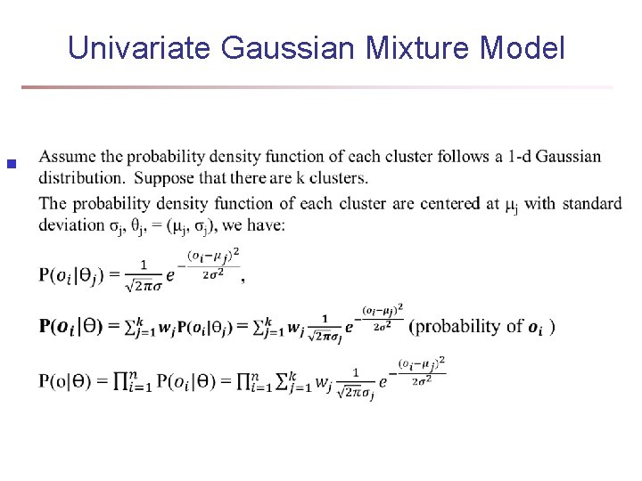
Univariate Gaussian Mixture Model n

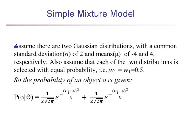
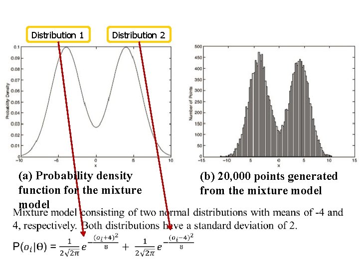
Simple Mixture Model n

Distribution 1 Distribution 2 (a) Probability density function for the mixture model (b) 20, 000 points generated from the mixture model

Univariate Gaussian Mixture Model n

EM algorithm n

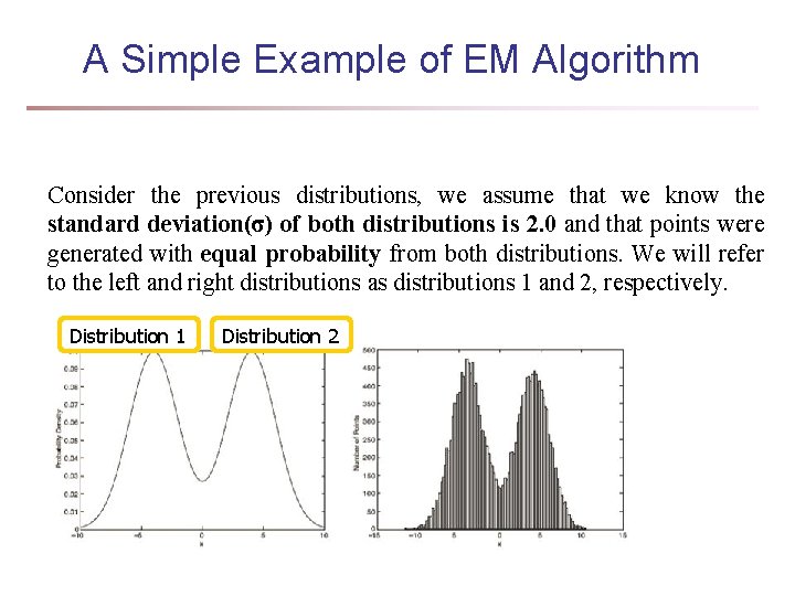
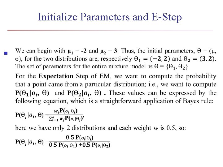
A Simple Example of EM Algorithm Consider the previous distributions, we assume that we know the standard deviation(σ) of both distributions is 2. 0 and that points were generated with equal probability from both distributions. We will refer to the left and right distributions as distributions 1 and 2, respectively. Distribution 1 Distribution 2

Initialize Parameters and E-Step n

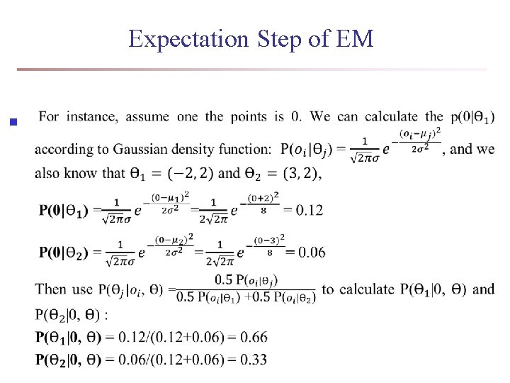
Expectation Step of EM n

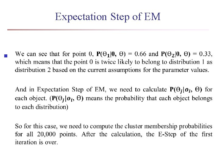
Expectation Step of EM n

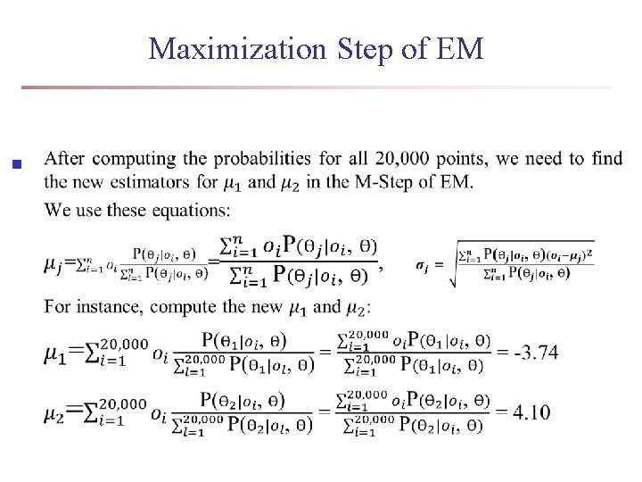
Maximization Step of EM n

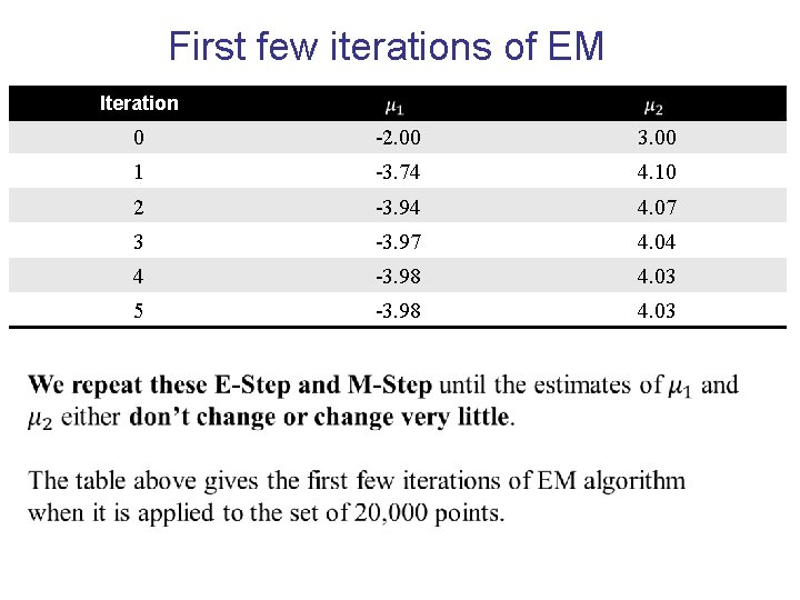
First few iterations of EM Iteration 0 -2. 00 3. 00 1 -3. 74 4. 10 2 -3. 94 4. 07 3 -3. 97 4. 04 4 -3. 98 4. 03 5 -3. 98 4. 03

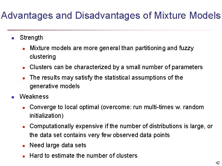
Advantages and Disadvantages of Mixture Models n Strength n n Mixture models are more general than partitioning and fuzzy clustering Clusters can be characterized by a small number of parameters The results may satisfy the statistical assumptions of the generative models Weakness n n Converge to local optimal (overcome: run multi-times w. random initialization) Computationally expensive if the number of distributions is large, or the data set contains very few observed data points n Need large data sets n Hard to estimate the number of clusters 42

Chapter 11. Cluster Analysis: Advanced Methods n Probability Model-Based Clustering n Clustering High-Dimensional Data n Clustering Graphs and Network Data n Clustering with Constraints n Summary 43

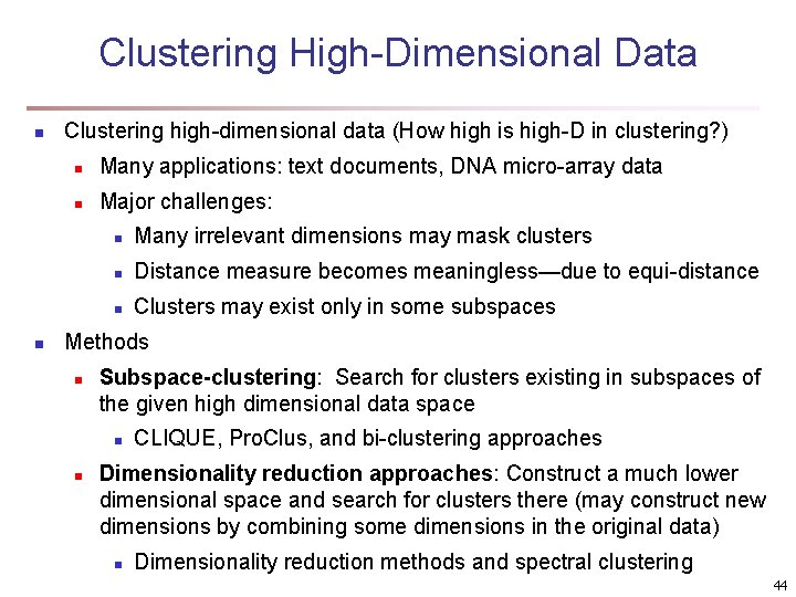
Clustering High-Dimensional Data n n Clustering high-dimensional data (How high is high-D in clustering? ) n Many applications: text documents, DNA micro-array data n Major challenges: n Many irrelevant dimensions may mask clusters n Distance measure becomes meaningless—due to equi-distance n Clusters may exist only in some subspaces Methods n Subspace-clustering: Search for clusters existing in subspaces of the given high dimensional data space n n CLIQUE, Pro. Clus, and bi-clustering approaches Dimensionality reduction approaches: Construct a much lower dimensional space and search for clusters there (may construct new dimensions by combining some dimensions in the original data) n Dimensionality reduction methods and spectral clustering 44

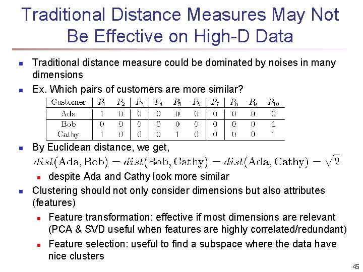
Traditional Distance Measures May Not Be Effective on High-D Data n Traditional distance measure could be dominated by noises in many dimensions Ex. Which pairs of customers are more similar? n By Euclidean distance, we get, n despite Ada and Cathy look more similar Clustering should not only consider dimensions but also attributes (features) n Feature transformation: effective if most dimensions are relevant (PCA & SVD useful when features are highly correlated/redundant) n Feature selection: useful to find a subspace where the data have nice clusters n n 45

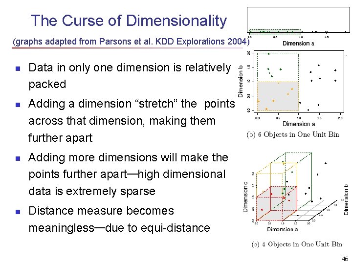
The Curse of Dimensionality (graphs adapted from Parsons et al. KDD Explorations 2004) n n Data in only one dimension is relatively packed Adding a dimension “stretch” the points across that dimension, making them further apart Adding more dimensions will make the points further apart—high dimensional data is extremely sparse Distance measure becomes meaningless—due to equi-distance 46

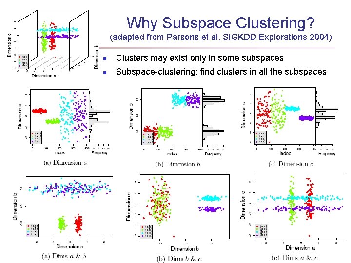
Why Subspace Clustering? (adapted from Parsons et al. SIGKDD Explorations 2004) n Clusters may exist only in some subspaces n Subspace-clustering: find clusters in all the subspaces 47

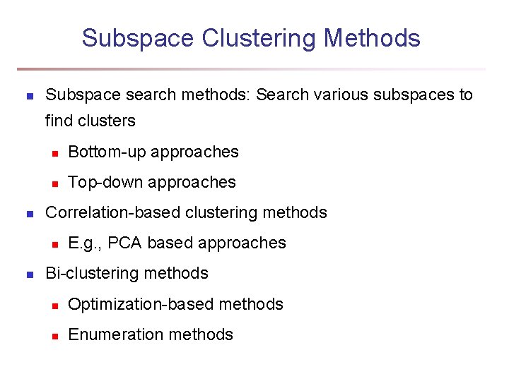
Subspace Clustering Methods n Subspace search methods: Search various subspaces to find clusters n n Bottom-up approaches n Top-down approaches Correlation-based clustering methods n n E. g. , PCA based approaches Bi-clustering methods n Optimization-based methods n Enumeration methods

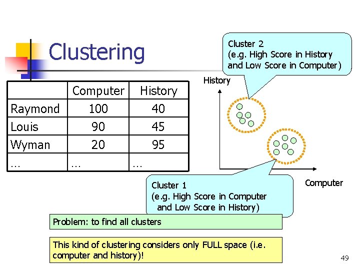
Clustering Raymond Louis Wyman Computer 100 90 20 … … Cluster 2 (e. g. High Score in History and Low Score in Computer) History 40 45 95 History … Cluster 1 (e. g. High Score in Computer and Low Score in History) Computer Problem: to find all clusters This kind of clustering considers only FULL space (i. e. computer and history)! COMP 5331 49

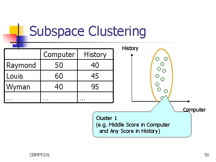
Subspace Clustering Raymond Louis Wyman Computer 50 60 40 … … History 40 45 95 History … Computer Cluster 1 (e. g. Middle Score in Computer and Any Score in History) COMP 5331 50

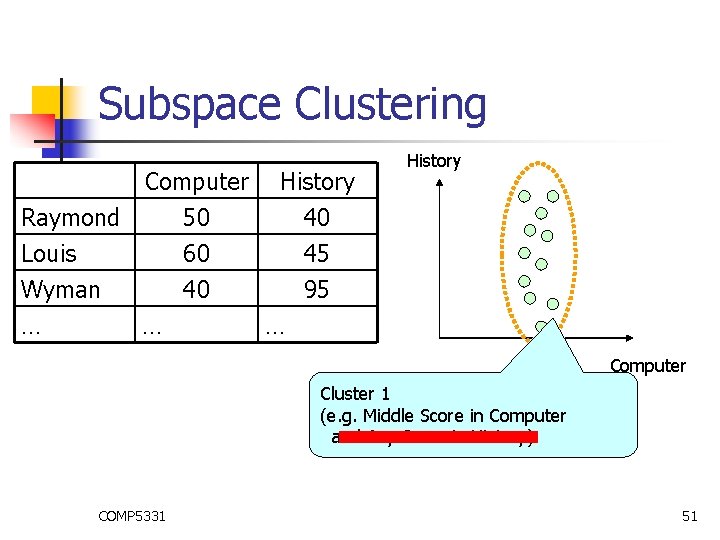
Subspace Clustering Raymond Louis Wyman Computer 50 60 40 … … History 40 45 95 History … Computer Cluster 1 (e. g. Middle Score in Computer and Any Score in History) COMP 5331 51

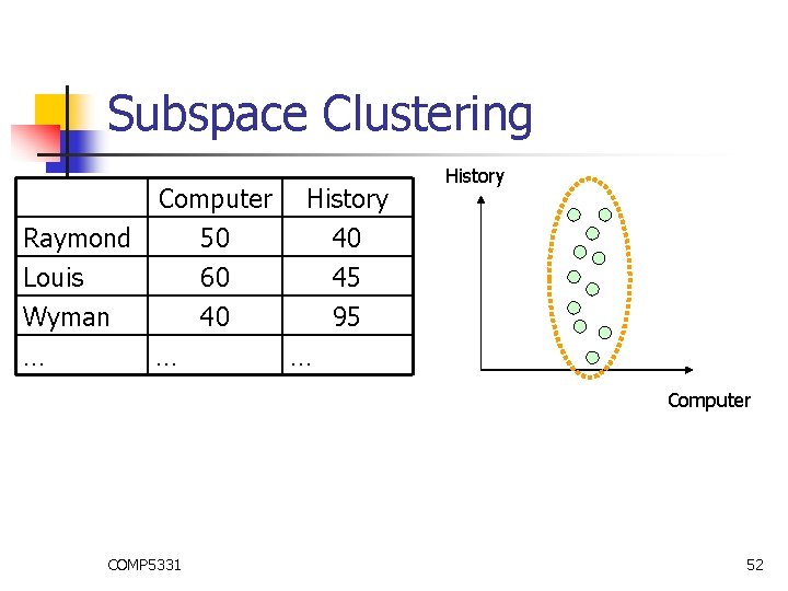
Subspace Clustering Raymond Louis Wyman Computer 50 60 40 … … History 40 45 95 History … Computer COMP 5331 52

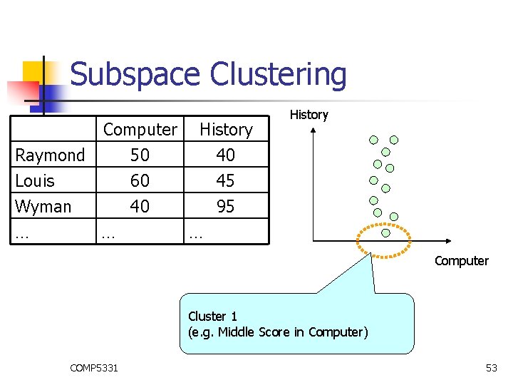
Subspace Clustering Raymond Louis Wyman Computer 50 60 40 … … History 40 45 95 History … Computer Cluster 1 (e. g. Middle Score in Computer) COMP 5331 53

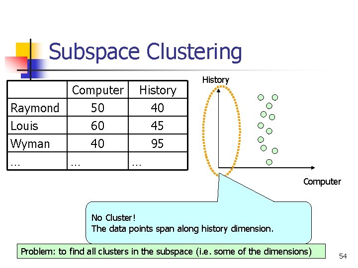
Subspace Clustering Raymond Louis Wyman Computer 50 60 40 … … History 40 45 95 History … Computer No Cluster! The data points span along history dimension. Problem: to find all clusters in the subspace (i. e. some of the dimensions) COMP 5331 54

Why Subspace Clustering? n Clustering for Understanding n Applications n Biology n n Psychology and Medicine n n Group different types of traffic patterns Software n COMP 5331 Group different customers for marketing Network n n Group medicine Business n n Group different species Group different programs for data analysis 55

Curse of Dimensionality n When the number of dimensions increases, n the distance between any two points is nearly the same Surprising results! This is the reason why we need to study subspace clustering COMP 5331 56

Subspace Clustering Methods n n n Dense Unit-based Method Entropy-Based Method Transformation-Based Method COMP 5331 57

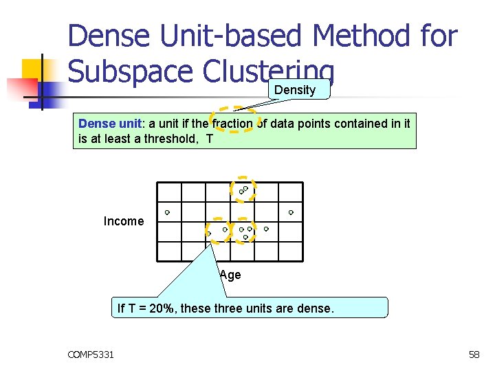
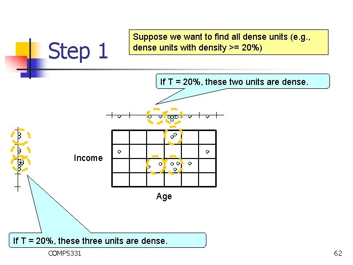
Dense Unit-based Method for Subspace Clustering Density Dense unit: a unit if the fraction of data points contained in it is at least a threshold, T Income Age If T = 20%, these three units are dense. COMP 5331 58

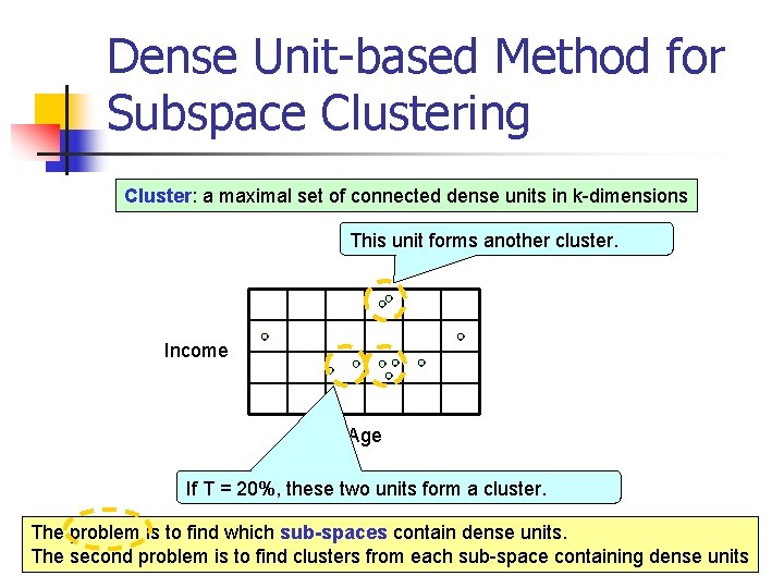
Dense Unit-based Method for Subspace Clustering Cluster: a maximal set of connected dense units in k-dimensions This unit forms another cluster. Income Age If T = 20%, these two units form a cluster. The problem is to find which sub-spaces contain dense units. The second problem is to find clusters from each sub-space containing dense units COMP 5331 59

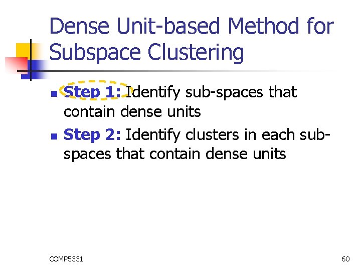
Dense Unit-based Method for Subspace Clustering n n Step 1: Identify sub-spaces that contain dense units Step 2: Identify clusters in each subspaces that contain dense units COMP 5331 60

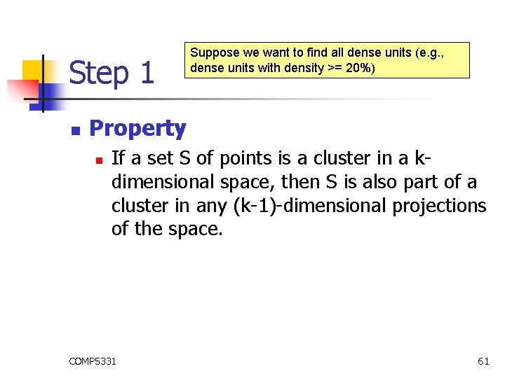
Step 1 n Suppose we want to find all dense units (e. g. , dense units with density >= 20%) Property n If a set S of points is a cluster in a kdimensional space, then S is also part of a cluster in any (k-1)-dimensional projections of the space. COMP 5331 61

Step 1 Suppose we want to find all dense units (e. g. , dense units with density >= 20%) If T = 20%, these two units are dense. Income Age If T = 20%, these three units are dense. COMP 5331 62

Step 1 n Suppose we want to find all dense units (e. g. , dense units with density >= 20%) We can make use of apriori approach to solve the problem COMP 5331 63

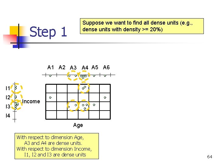
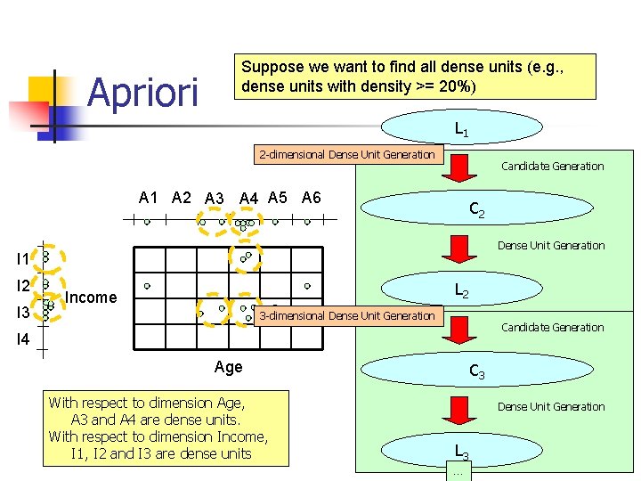
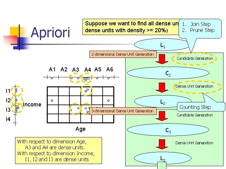
Step 1 Suppose we want to find all dense units (e. g. , dense units with density >= 20%) A 1 A 2 A 3 A 4 A 5 A 6 I 1 I 2 I 3 Income I 4 Age With respect to dimension Age, A 3 and A 4 are dense units. With respect to dimension Income, I 1, I 2 and I 3 are dense units COMP 5331 64

Apriori Suppose we want to find all dense units (e. g. , dense units with density >= 20%) L 1 2 -dimensional Dense Unit Generation Candidate Generation A 1 A 2 A 3 A 4 A 5 A 6 C 2 Dense Unit Generation I 1 I 2 I 3 L 2 Income 3 -dimensional Dense Unit Generation Candidate Generation I 4 Age With respect to dimension Age, A 3 and A 4 are dense units. With respect to dimension Income, I 1, I 2 and I 3 are dense units COMP 5331 C 3 Dense Unit Generation L 3 … 65

Apriori Suppose we want to find all dense units (e. g. , 1. Join Step 2. Prune Step dense units with density >= 20%) L 1 2 -dimensional Dense Unit Generation Candidate Generation A 1 A 2 A 3 A 4 A 5 A 6 C 2 Dense Unit Generation I 1 I 2 I 3 L 2 Income Counting Step 3 -dimensional Dense Unit Generation Candidate Generation I 4 Age With respect to dimension Age, A 3 and A 4 are dense units. With respect to dimension Income, I 1, I 2 and I 3 are dense units COMP 5331 C 3 Dense Unit Generation L 3 … 66

Dense Unit-based Method for Subspace Clustering n n Step 1: Identify sub-spaces that contain dense units Step 2: Identify clusters in each subspaces that contain dense units COMP 5331 67

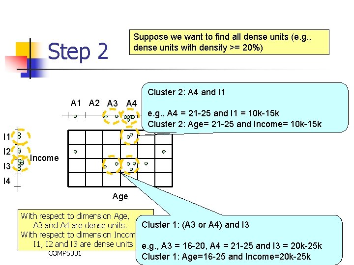
Suppose we want to find all dense units (e. g. , dense units with density >= 20%) Step 2 Cluster 2: A 4 and I 1 A 2 A 3 A 4 A 5 A 6 e. g. , A 4 = 21 -25 and I 1 = 10 k-15 k Cluster 2: Age= 21 -25 and Income= 10 k-15 k I 1 I 2 I 3 Income I 4 Age With respect to dimension Age, Cluster 1: (A 3 or A 4) and I 3 A 3 and A 4 are dense units. With respect to dimension Income, I 1, I 2 and I 3 are dense units e. g. , A 3 = 16 -20, A 4 = 21 -25 and I 3 = 20 k-25 k COMP 5331 Cluster 1: Age=16 -25 and Income=20 k-25 k 68

Subspace Clustering Methods n n n Dense Unit-based Method Entropy-Based Method Transformation-Based Method COMP 5331 69

Entropy-Based Method for Subspace Clustering n n Entropy Problem n n Good subspace Clustering Algorithm n n Property Apriori COMP 5331 70

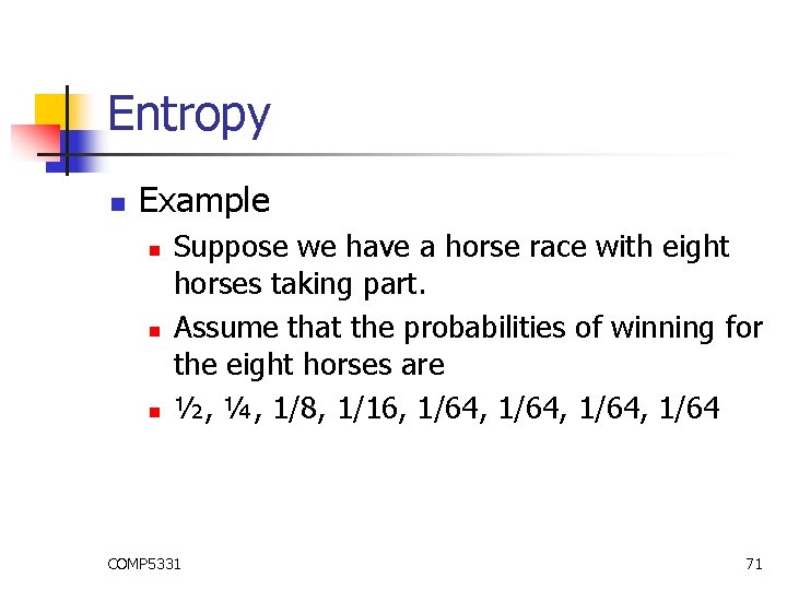
Entropy n Example n n n Suppose we have a horse race with eight horses taking part. Assume that the probabilities of winning for the eight horses are ½, ¼, 1/8, 1/16, 1/64, 1/64 COMP 5331 71

Entropy n Suppose we want to send a message to another person indicating which horse won the race. One method is to send a 3 bit string to denote the index of the winning horse COMP 5331 72

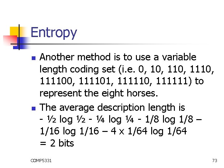
Entropy n n Another method is to use a variable length coding set (i. e. 0, 110, 1110, 111100, 111101, 111110, 111111) to represent the eight horses. The average description length is - ½ log ½ - ¼ log ¼ - 1/8 log 1/8 – 1/16 log 1/16 – 4 x 1/64 log 1/64 = 2 bits COMP 5331 73

Entropy n n The entropy is a way to measure the amount of information. The smaller the entropy (viewed as the average length of description length in the above example), the more informative we have. COMP 5331 74

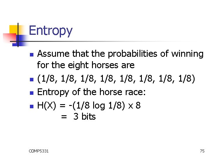
Entropy n n Assume that the probabilities of winning for the eight horses are (1/8, 1/8, 1/8) Entropy of the horse race: H(X) = -(1/8 log 1/8) x 8 = 3 bits COMP 5331 75

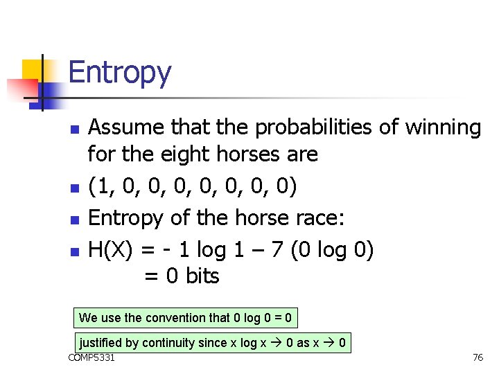
Entropy n n Assume that the probabilities of winning for the eight horses are (1, 0, 0, 0, 0) Entropy of the horse race: H(X) = - 1 log 1 – 7 (0 log 0) = 0 bits We use the convention that 0 log 0 = 0 justified by continuity since x log x 0 as x 0 COMP 5331 76

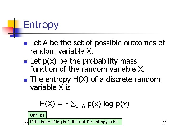
Entropy n n n Let A be the set of possible outcomes of random variable X. Let p(x) be the probability mass function of the random variable X. The entropy H(X) of a discrete random variable X is H(X) = - x A p(x) log p(x) Unit: bit If the base of log is 2, the unit for entropy is bit. COMP 5331 77

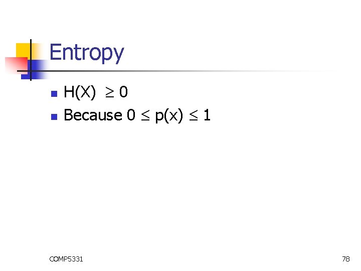
Entropy n n H(X) 0 Because 0 p(x) 1 COMP 5331 78

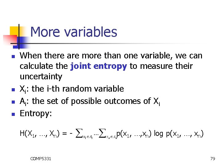
More variables n n When there are more than one variable, we can calculate the joint entropy to measure their uncertainty Xi: the i-th random variable Ai: the set of possible outcomes of Xi Entropy: H(X 1, …, Xn) = - p(x 1, …, xn) log p(x 1, …, xn) COMP 5331 79

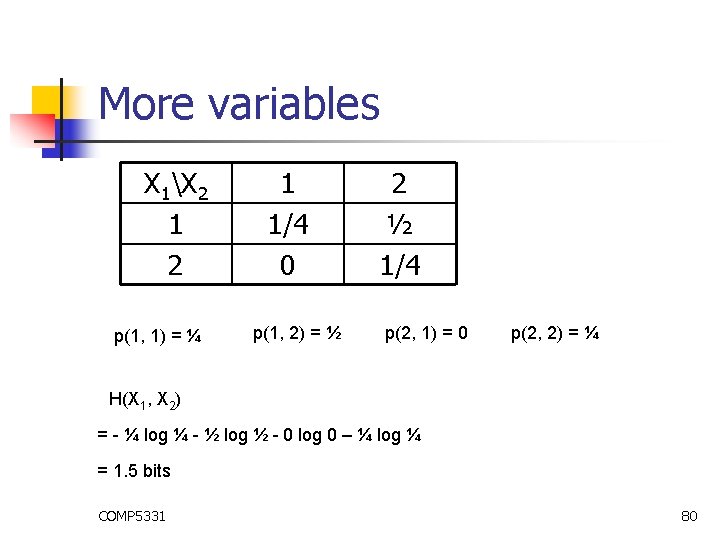
More variables X 1X 2 1 2 p(1, 1) = ¼ 1 1/4 0 p(1, 2) = ½ 2 ½ 1/4 p(2, 1) = 0 p(2, 2) = ¼ H(X 1, X 2) = - ¼ log ¼ - ½ log ½ - 0 log 0 – ¼ log ¼ = 1. 5 bits COMP 5331 80

Entropy-Based Method for Subspace Clustering n n Entropy Problem n n Good subspace Clustering Algorithm n n Property Apriori COMP 5331 81

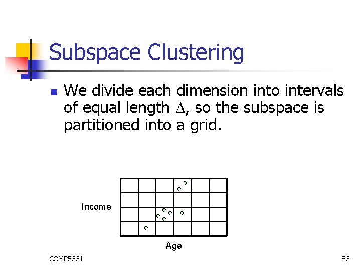
Subspace Clustering n We divide each dimension into intervals of equal length , so the subspace is partitioned into a grid. COMP 5331 82

Subspace Clustering n We divide each dimension into intervals of equal length , so the subspace is partitioned into a grid. Income Age COMP 5331 83

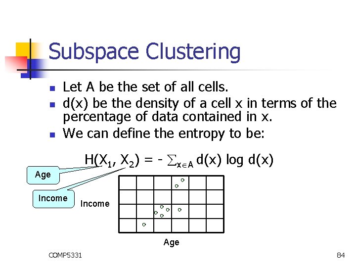
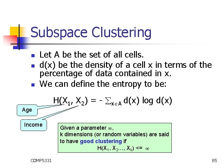
Subspace Clustering n n n Age Let A be the set of all cells. d(x) be the density of a cell x in terms of the percentage of data contained in x. We can define the entropy to be: H(X 1, X 2) = - x A d(x) log d(x) Income Age COMP 5331 84

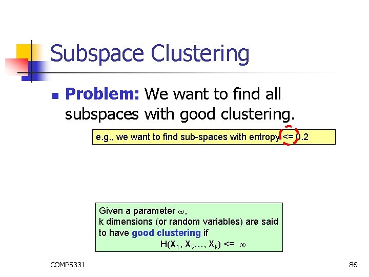
Subspace Clustering n n n Age Let A be the set of all cells. d(x) be the density of a cell x in terms of the percentage of data contained in x. We can define the entropy to be: H(X 1, X 2) = - x A d(x) log d(x) Income COMP 5331 Given a parameter , k dimensions (or random variables) are said to have good clustering if H(X 1, X 2…, Xk) <= 85

Subspace Clustering n Problem: We want to find all subspaces with good clustering. e. g. , we want to find sub-spaces with entropy <= 0. 2 Given a parameter , k dimensions (or random variables) are said to have good clustering if H(X 1, X 2…, Xk) <= COMP 5331 86

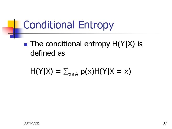
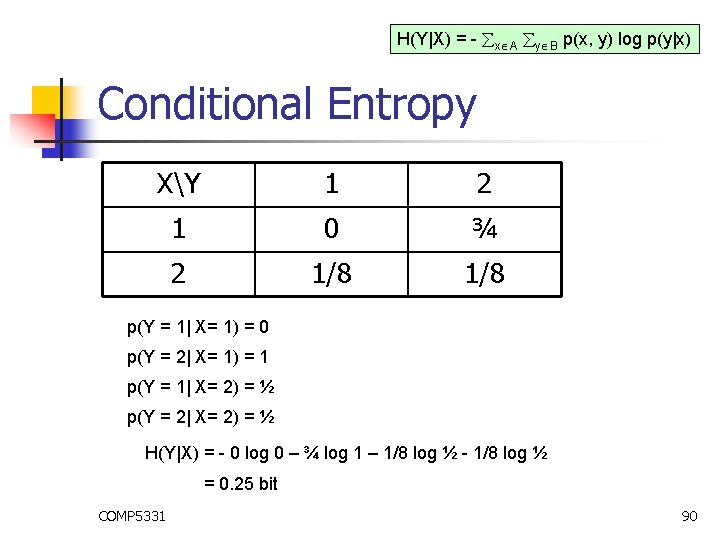
Conditional Entropy n The conditional entropy H(Y|X) is defined as H(Y|X) = x A p(x)H(Y|X = x) COMP 5331 87

Conditional Entropy XY 1 2 1 0 ¾ 2 1/8 H(Y|X=1) = 0 bit H(Y|X=2) = 1 bit H(Y|X) = ¾ x H(Y|X=1) + ¼ x. H(Y|X = 2) = 0. 25 bit COMP 5331 88

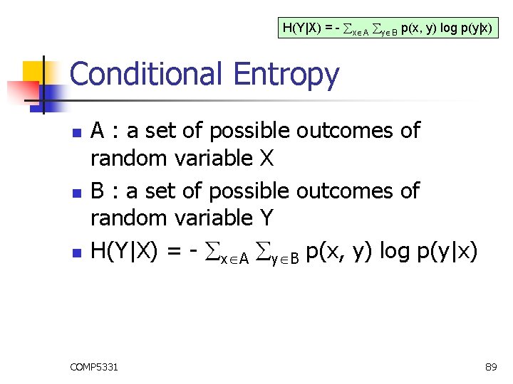
H(Y|X) = - x A y B p(x, y) log p(y|x) Conditional Entropy n n n A : a set of possible outcomes of random variable X B : a set of possible outcomes of random variable Y H(Y|X) = - x A y B p(x, y) log p(y|x) COMP 5331 89

H(Y|X) = - x A y B p(x, y) log p(y|x) Conditional Entropy XY 1 2 1 0 ¾ 2 1/8 p(Y = 1| X= 1) = 0 p(Y = 2| X= 1) = 1 p(Y = 1| X= 2) = ½ p(Y = 2| X= 2) = ½ H(Y|X) = - 0 log 0 – ¾ log 1 – 1/8 log ½ - 1/8 log ½ = 0. 25 bit COMP 5331 90

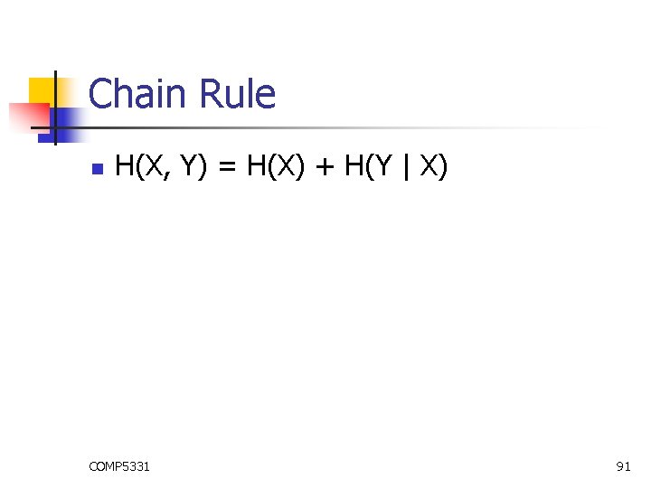
Chain Rule n H(X, Y) = H(X) + H(Y | X) COMP 5331 91

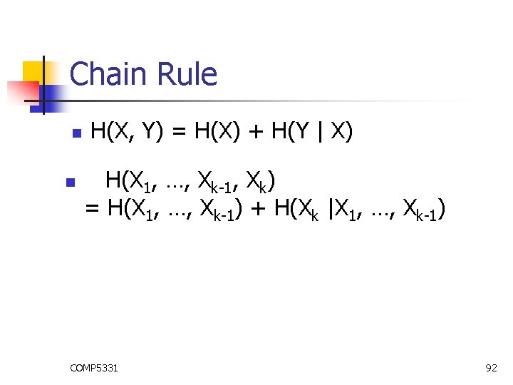
Chain Rule n n H(X, Y) = H(X) + H(Y | X) H(X 1, …, Xk-1, Xk) = H(X 1, …, Xk-1) + H(Xk |X 1, …, Xk-1) COMP 5331 92

Entropy-Based Method for Subspace Clustering n n Entropy Problem n n Good subspace Clustering Algorithm n n Property Apriori COMP 5331 93

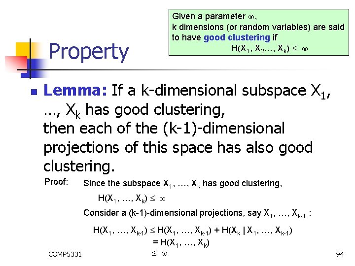
Property n Given a parameter , k dimensions (or random variables) are said to have good clustering if H(X 1, X 2…, Xk) Lemma: If a k-dimensional subspace X 1, …, Xk has good clustering, then each of the (k-1)-dimensional projections of this space has also good clustering. Proof: Since the subspace X 1, …, Xk has good clustering, H(X 1, …, Xk) Consider a (k-1)-dimensional projections, say X 1, …, Xk-1 : COMP 5331 H(X 1, …, Xk-1) + H(Xk | X 1, …, Xk-1) = H(X 1, …, Xk) 94

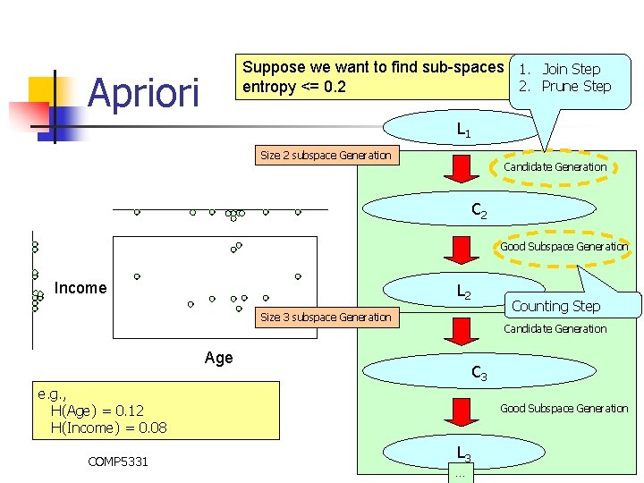
Apriori n Suppose we want to find sub-spaces with entropy <= 0. 2 We can make use of apriori approach to solve the problem COMP 5331 95

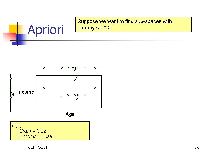
Suppose we want to find sub-spaces with entropy <= 0. 2 Apriori Income Age e. g. , H(Age) = 0. 12 H(Income) = 0. 08 COMP 5331 96

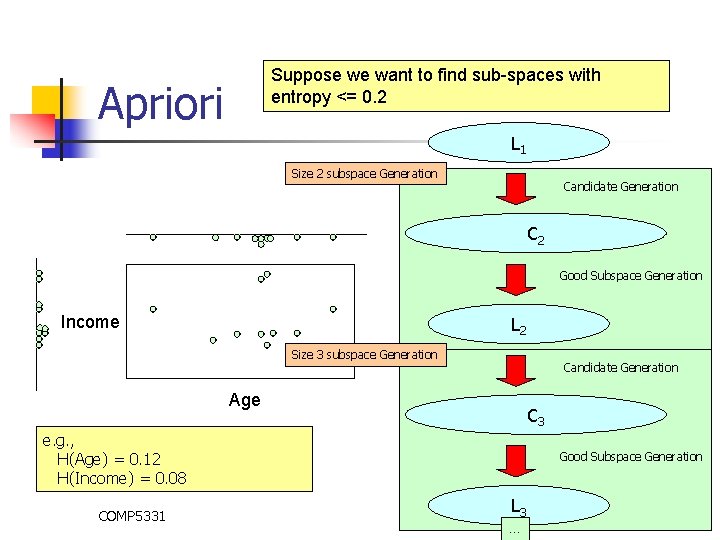
Suppose we want to find sub-spaces with entropy <= 0. 2 Apriori L 1 Size 2 subspace Generation Candidate Generation C 2 Good Subspace Generation Income L 2 Size 3 subspace Generation Candidate Generation Age C 3 e. g. , H(Age) = 0. 12 H(Income) = 0. 08 COMP 5331 Good Subspace Generation L 3 … 97

Suppose we want to find sub-spaces with 1. Join Step 2. Prune Step entropy <= 0. 2 Apriori L 1 Size 2 subspace Generation Candidate Generation C 2 Good Subspace Generation Income L 2 Counting Step Size 3 subspace Generation Candidate Generation Age C 3 e. g. , H(Age) = 0. 12 H(Income) = 0. 08 COMP 5331 Good Subspace Generation L 3 … 98

Cluster n n Suppose we want to find sub-spaces with entropy <= 0. 2 After finding the subspaces with entropy <= 0. 2, We can find the real clusters by existing methods (e. g. , k-mean) in each of the subspaces found. COMP 5331 99

Subspace Clustering Methods n n n Dense Unit-based Method Entropy-Based Method Transformation-Based Method COMP 5331 100

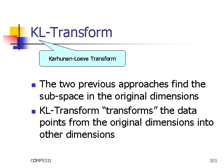
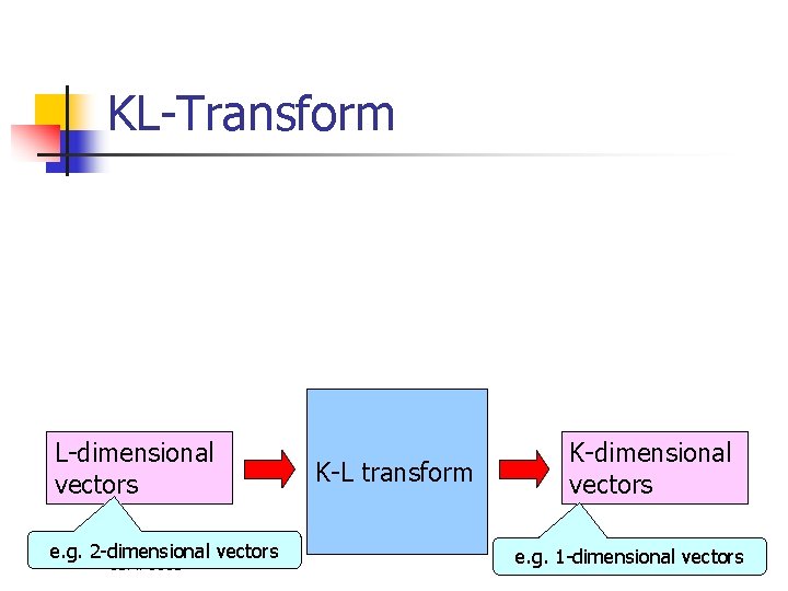
KL-Transform Karhunen-Loeve Transform n n The two previous approaches find the sub-space in the original dimensions KL-Transform “transforms” the data points from the original dimensions into other dimensions COMP 5331 101

KL-Transform L-dimensional vectors e. g. 2 -dimensional vectors COMP 5331 K-L transform K-dimensional vectors e. g. 1 -dimensional vectors 102

L-dimensional vectors e. g. 2 -dimensional vectors COMP 5331 K-L transform K-dimensional vectors e. g. 1 -dimensional vectors 103

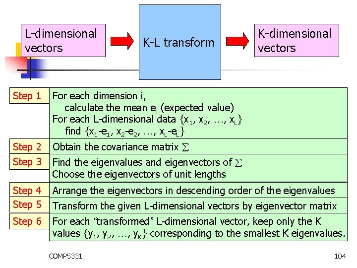
L-dimensional vectors K-L transform K-dimensional vectors Step 1 For each dimension i, calculate the mean ei (expected value) For each L-dimensional data {x 1, x 2, …, x. L} find {x 1 -e 1, x 2 -e 2, …, x. L-e. L} Step 2 Obtain the covariance matrix Step 3 Find the eigenvalues and eigenvectors of Choose the eigenvectors of unit lengths Step 4 Step 5 Arrange the eigenvectors in descending order of the eigenvalues Step 6 For each “transformed” L-dimensional vector, keep only the K values {y 1, y 2, …, y. K} corresponding to the smallest K eigenvalues. Transform the given L-dimensional vectors by eigenvector matrix COMP 5331 104

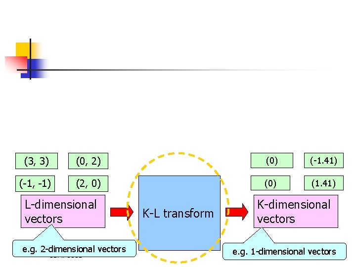
(3, 3) (0, 2) (0) (-1. 41) (-1, -1) (2, 0) (1. 41) L-dimensional vectors e. g. 2 -dimensional vectors COMP 5331 K-L transform K-dimensional vectors e. g. 1 -dimensional vectors 105

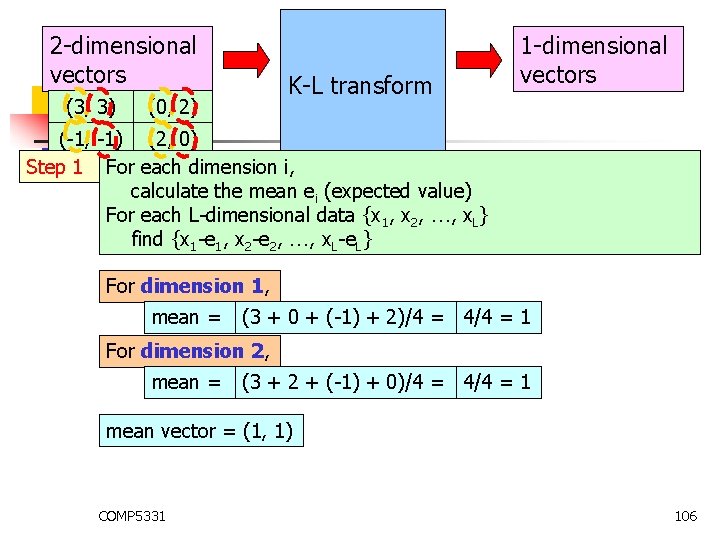
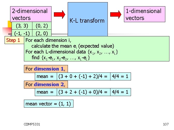
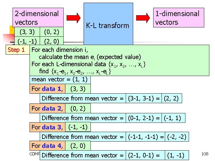
2 -dimensional vectors (3, 3) K-L transform (0, 2) 1 -dimensional vectors (-1, -1) (2, 0) Step 1 For each dimension i, calculate the mean ei (expected value) For each L-dimensional data {x 1, x 2, …, x. L} find {x 1 -e 1, x 2 -e 2, …, x. L-e. L} For dimension 1, mean = (3 + 0 + (-1) + 2)/4 = 4/4 = 1 For dimension 2, mean = (3 + 2 + (-1) + 0)/4 = 4/4 = 1 mean vector = (1, 1) COMP 5331 106

2 -dimensional vectors (3, 3) K-L transform (0, 2) 1 -dimensional vectors (-1, -1) (2, 0) Step 1 For each dimension i, calculate the mean ei (expected value) For each L-dimensional data {x 1, x 2, …, x. L} find {x 1 -e 1, x 2 -e 2, …, x. L-e. L} For dimension 1, mean = (3 + 0 + (-1) + 2)/4 = 4/4 = 1 For dimension 2, mean = (3 + 2 + (-1) + 0)/4 = 4/4 = 1 mean vector = (1, 1) COMP 5331 107

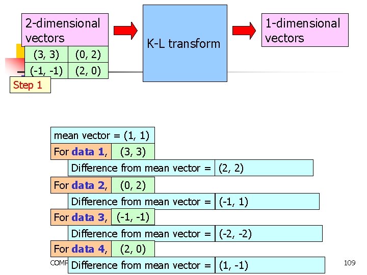
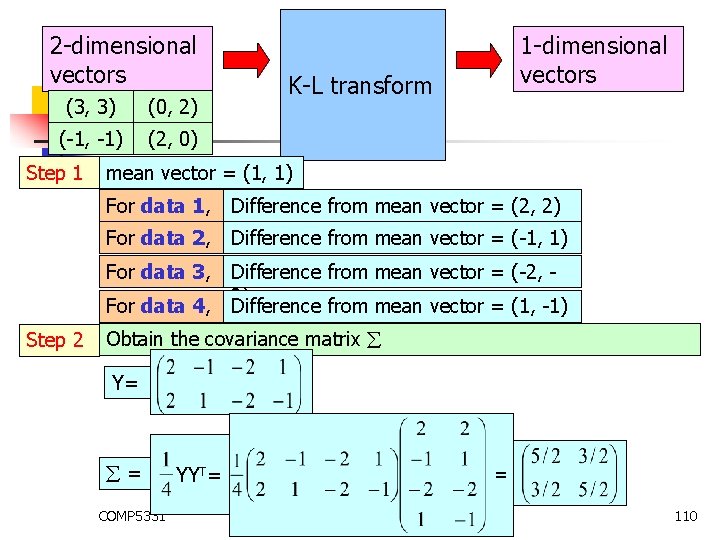
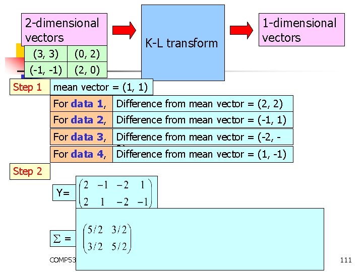
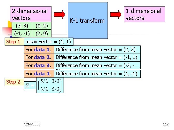
2 -dimensional vectors (3, 3) K-L transform (0, 2) 1 -dimensional vectors (-1, -1) (2, 0) Step 1 For each dimension i, calculate the mean ei (expected value) For each L-dimensional data {x 1, x 2, …, x. L} find {x 1 -e 1, x 2 -e 2, …, x. L-e. L} mean vector = (1, 1) For data 1, (3, 3) Difference from mean vector = (3 -1, 3 -1) = (2, 2) For data 2, (0, 2) Difference from mean vector = (0 -1, 2 -1) = (-1, 1) For data 3, (-1, -1) Difference from mean vector = (-1 -1, -1 -1) = (-2, -2) For data 4, (2, 0) COMP 5331 Difference from mean vector = (2 -1, 0 -1) = (1, -1) 108

2 -dimensional vectors (3, 3) (-1, -1) Step 1 K-L transform (0, 2) 1 -dimensional vectors (2, 0) mean vector = (1, 1) For data 1, (3, 3) (2, 2) Difference from mean vector = (3 -1, 3 -1) = (2, 2) For data 2, (0, 2) Difference from mean vector = (0 -1, 2 -1) = (-1, 1) For data 3, (-1, -1) Difference from mean vector = (-1 -1, -1 -1) = (-2, -2) For data 4, (2, 0) COMP 5331 Difference from mean vector = (2 -1, 0 -1) = (1, -1) 109

2 -dimensional vectors (3, 3) (0, 2) (-1, -1) (2, 0) Step 1 K-L transform mean vector = (1, 1) For data 1, Difference from mean vector = (2, 2) For data 2, Difference from mean vector = (-1, 1) For data 3, Difference from mean vector = (-2, 2) Difference from mean vector = (1, -1) For data 4, Step 2 1 -dimensional vectors Obtain the covariance matrix Y= = YYT= COMP 5331 = 110

2 -dimensional vectors (3, 3) (0, 2) (-1, -1) (2, 0) Step 1 1 -dimensional vectors K-L transform mean vector = (1, 1) For data 1, Difference from mean vector = (2, 2) For data 2, Difference from mean vector = (-1, 1) For data 3, Difference from mean vector = (-2, 2) Difference from mean vector = (1, -1) For data 4, Step 2 Y= = YYT= COMP 5331 = 111

2 -dimensional vectors (3, 3) (0, 2) (-1, -1) (2, 0) Step 1 mean vector = (1, 1) For data 1, Difference from mean vector = (2, 2) For data 2, Difference from mean vector = (-1, 1) For data 3, Difference from mean vector = (-2, 2) Difference from mean vector = (1, -1) For data 4, Step 2 K-L transform 1 -dimensional vectors = COMP 5331 112

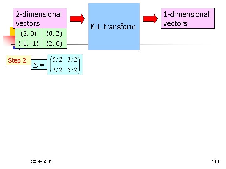
2 -dimensional vectors (3, 3) (0, 2) (-1, -1) (2, 0) Step 2 K-L transform 1 -dimensional vectors = COMP 5331 113

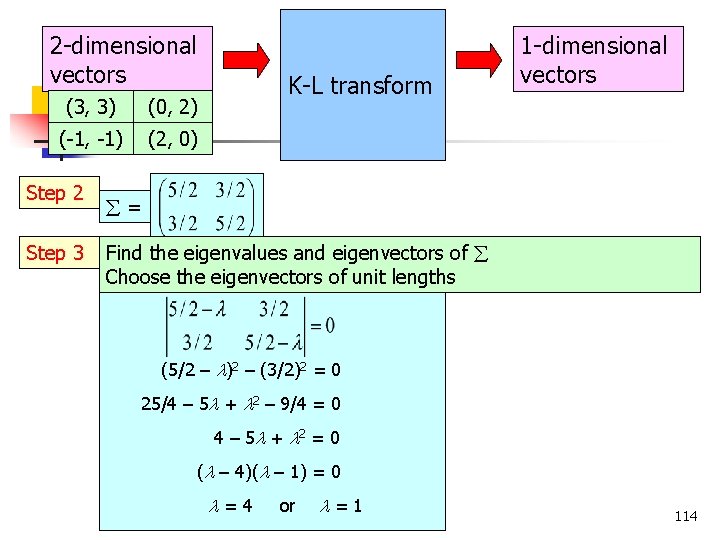
2 -dimensional vectors (3, 3) (0, 2) (-1, -1) (2, 0) Step 2 Step 3 K-L transform 1 -dimensional vectors = Find the eigenvalues and eigenvectors of Choose the eigenvectors of unit lengths (5/2 – )2 – (3/2)2 = 0 25/4 – 5 + 2 – 9/4 = 0 4 – 5 + 2 = 0 ( – 4)( – 1) = 0 COMP 5331 = 4 or = 1 114

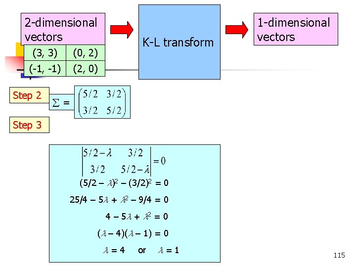
2 -dimensional vectors (3, 3) (0, 2) (-1, -1) (2, 0) Step 2 K-L transform 1 -dimensional vectors = Step 3 (5/2 – )2 – (3/2)2 = 0 25/4 – 5 + 2 – 9/4 = 0 4 – 5 + 2 = 0 ( – 4)( – 1) = 0 COMP 5331 = 4 or = 1 115

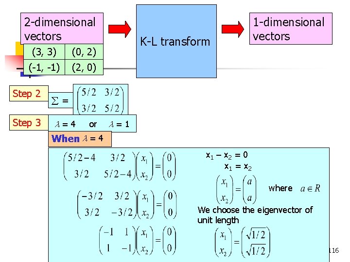
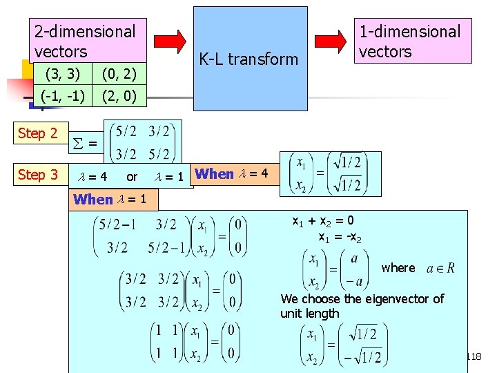
2 -dimensional vectors (3, 3) (0, 2) (-1, -1) (2, 0) Step 2 Step 3 K-L transform 1 -dimensional vectors = = 4 or = 1 When = 4 x 1 – x 2 = 0 x 1 = x 2 where We choose the eigenvector of unit length COMP 5331 116

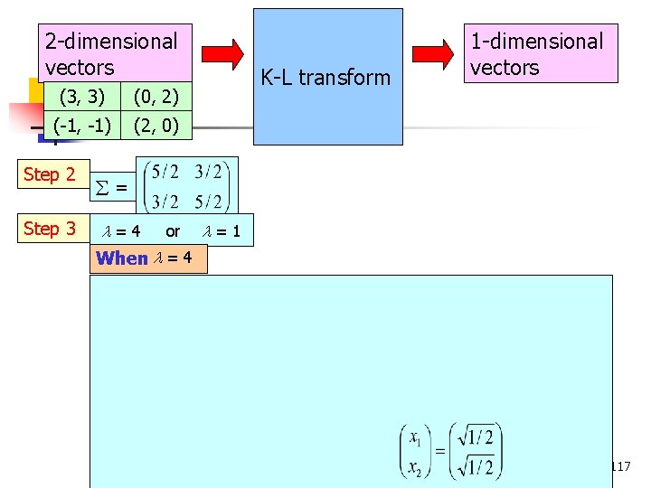
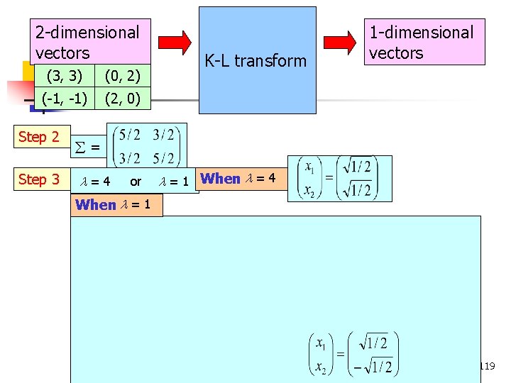
2 -dimensional vectors (3, 3) (0, 2) (-1, -1) (2, 0) Step 2 Step 3 K-L transform 1 -dimensional vectors = = 4 or = 1 When = 4 COMP 5331 117

2 -dimensional vectors (3, 3) (0, 2) (-1, -1) (2, 0) Step 2 Step 3 K-L transform 1 -dimensional vectors = = 4 or = 1 When = 4 When = 1 x 1 + x 2 = 0 x 1 = -x 2 where We choose the eigenvector of unit length COMP 5331 118

2 -dimensional vectors (3, 3) (0, 2) (-1, -1) (2, 0) Step 2 Step 3 K-L transform 1 -dimensional vectors = = 4 or = 1 When = 4 When = 1 COMP 5331 119

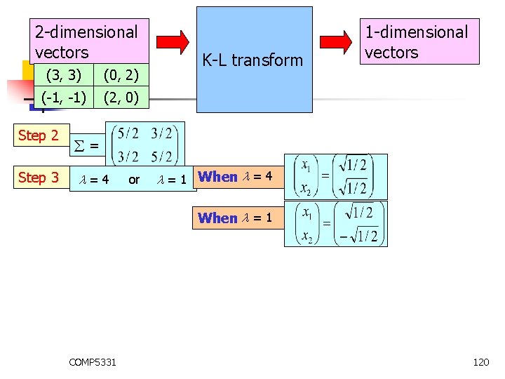
2 -dimensional vectors (3, 3) (0, 2) (-1, -1) (2, 0) Step 2 Step 3 K-L transform 1 -dimensional vectors = = 4 or = 1 When = 4 When = 1 COMP 5331 120

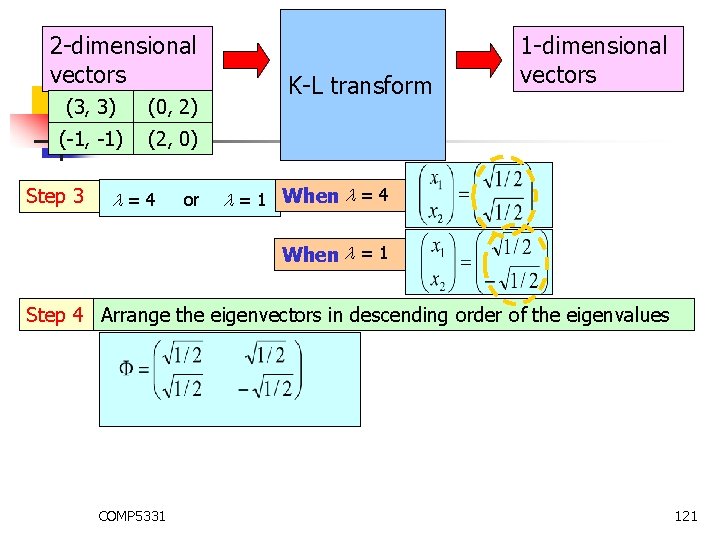
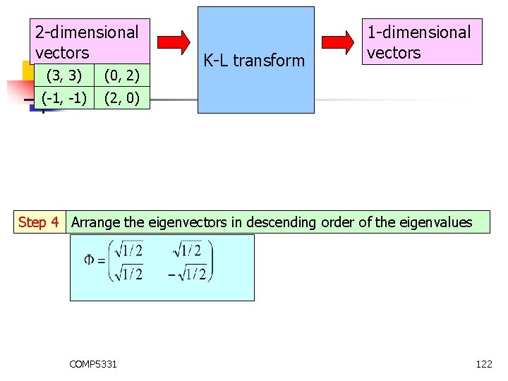
2 -dimensional vectors (3, 3) (0, 2) (-1, -1) (2, 0) Step 3 K-L transform 1 -dimensional vectors = 4 or = 1 When = 4 When = 1 Step 4 Arrange the eigenvectors in descending order of the eigenvalues COMP 5331 121

2 -dimensional vectors (3, 3) (0, 2) (-1, -1) (2, 0) K-L transform 1 -dimensional vectors Step 4 Arrange the eigenvectors in descending order of the eigenvalues COMP 5331 122

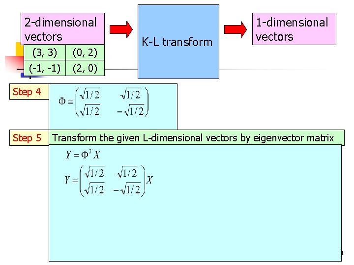
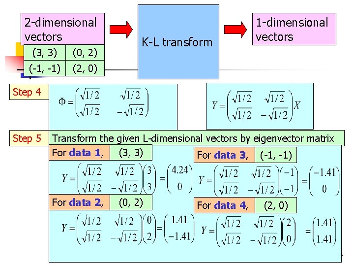
2 -dimensional vectors (3, 3) (0, 2) (-1, -1) (2, 0) K-L transform 1 -dimensional vectors Step 4 Step 5 Transform the given L-dimensional vectors by eigenvector matrix COMP 5331 123

2 -dimensional vectors (3, 3) (0, 2) (-1, -1) (2, 0) K-L transform 1 -dimensional vectors Step 4 Step 5 Transform the given L-dimensional vectors by eigenvector matrix COMP 5331 124

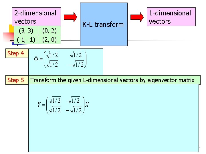
2 -dimensional vectors (3, 3) (0, 2) (-1, -1) (2, 0) K-L transform 1 -dimensional vectors Step 4 Step 5 Transform the given L-dimensional vectors by eigenvector matrix COMP 5331 125

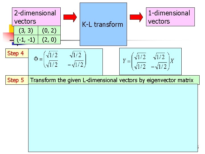
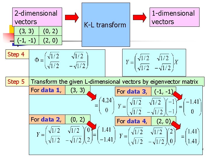
2 -dimensional vectors (3, 3) (0, 2) (-1, -1) (2, 0) K-L transform 1 -dimensional vectors Step 4 Step 5 Transform the given L-dimensional vectors by eigenvector matrix (3, 3) For data 1, For data 3, (-1, -1) For data 2, COMP 5331 (0, 2) For data 4, (2, 0) 126

2 -dimensional vectors (3, 3) (0, 2) (-1, -1) (2, 0) K-L transform 1 -dimensional vectors Step 4 Step 5 Transform the given L-dimensional vectors by eigenvector matrix (3, 3) For data 1, For data 3, (-1, -1) For data 2, COMP 5331 (0, 2) For data 4, (2, 0) 127

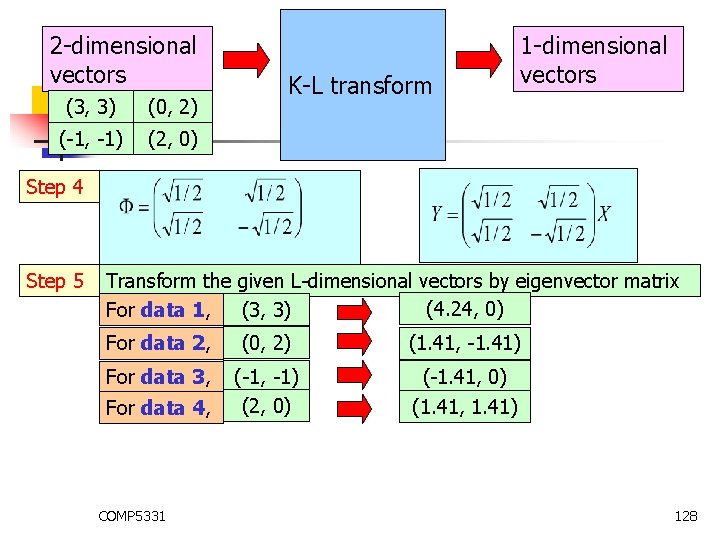
2 -dimensional vectors (3, 3) (0, 2) (-1, -1) (2, 0) K-L transform 1 -dimensional vectors Step 4 Step 5 Transform the given L-dimensional vectors by eigenvector matrix (4. 24, 0) (3, 3) For data 1, For data 2, (0, 2) (1. 41, -1. 41) For data 3, (-1, -1) (2, 0) (-1. 41, 0) For data 4, COMP 5331 (1. 41, 1. 41) 128

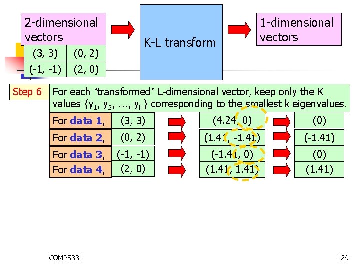
2 -dimensional vectors (3, 3) (0, 2) (-1, -1) (2, 0) Step 6 K-L transform 1 -dimensional vectors For each “transformed” L-dimensional vector, keep only the K values {y 1, y 2, …, y. K} corresponding to the smallest k eigenvalues. For data 1, (3, 3) (4. 24, 0) (0) For data 2, (0, 2) (1. 41, -1. 41) (-1. 41) For data 3, (-1, -1) (2, 0) (-1. 41, 0) (1. 41, 1. 41) (1. 41) For data 4, COMP 5331 129

n n Why do we need to do this KLtransform? Why do we choose the eigenvectors with the smallest eigenvalues? COMP 5331 130

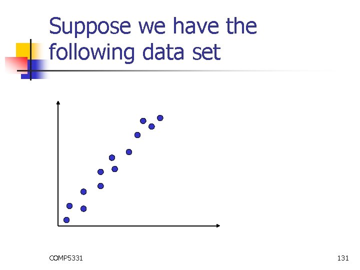
Suppose we have the following data set COMP 5331 131

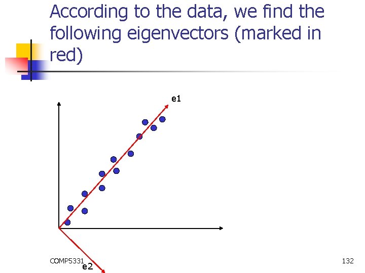
According to the data, we find the following eigenvectors (marked in red) e 1 COMP 5331 e 2 132

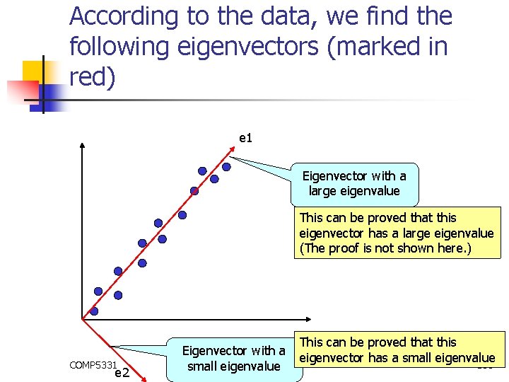
According to the data, we find the following eigenvectors (marked in red) e 1 Eigenvector with a large eigenvalue This can be proved that this eigenvector has a large eigenvalue (The proof is not shown here. ) COMP 5331 e 2 This can be proved that this Eigenvector with a eigenvector has a small eigenvalue 133 small eigenvalue

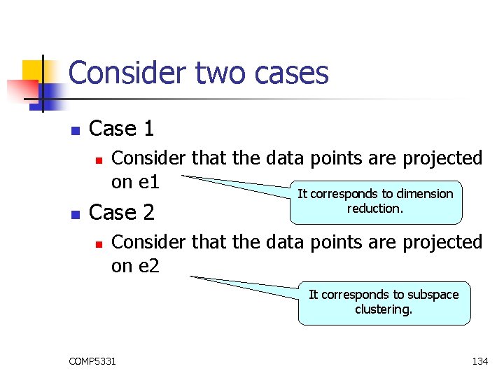
Consider two cases n Case 1 n n Consider that the data points are projected on e 1 It corresponds to dimension Case 2 n reduction. Consider that the data points are projected on e 2 It corresponds to subspace clustering. COMP 5331 134

Case 1 n Consider that the data points are projected on e 1 COMP 5331 135

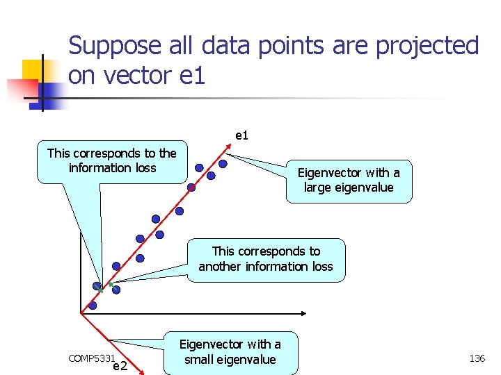
Suppose all data points are projected on vector e 1 This corresponds to the information loss Eigenvector with a large eigenvalue This corresponds to another information loss COMP 5331 e 2 Eigenvector with a small eigenvalue 136

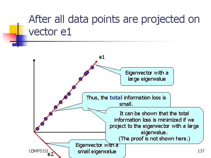
After all data points are projected on vector e 1 Eigenvector with a large eigenvalue Thus, the total information loss is small. COMP 5331 e 2 It can be shown that the total information loss is minimized if we project to the eigenvector with a large eigenvalue. (The proof is not shown here. ) Eigenvector with a 137 small eigenvalue

Objective of Dimension Reduction n The objective of Dimension Reduction n To reduce the total number of dimensions At the same time, we want to keep information as much as possible. (i. e. , minimize the information loss) In our example, n n n We reduce from two dimensions to one dimension The eigenvector with a large eigenvector corresponds to this dimension After we adopt this dimension, we can minimize the information loss COMP 5331 138

Case 2 n Consider that the data points are projected on e 2 COMP 5331 139

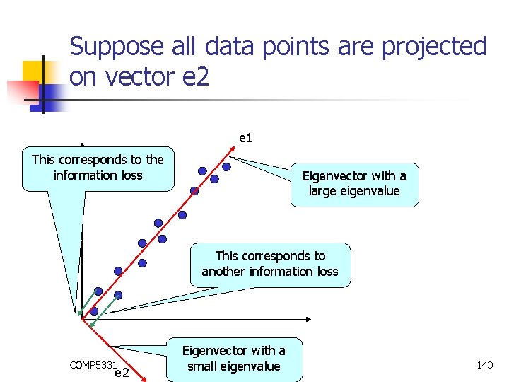
Suppose all data points are projected on vector e 2 e 1 This corresponds to the information loss Eigenvector with a large eigenvalue This corresponds to another information loss COMP 5331 e 2 Eigenvector with a small eigenvalue 140

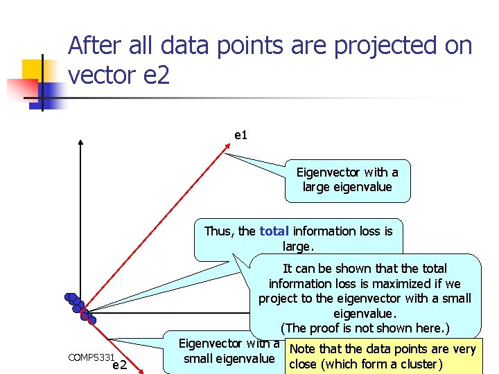
After all data points are projected on vector e 2 e 1 Eigenvector with a large eigenvalue Thus, the total information loss is large. COMP 5331 e 2 It can be shown that the total information loss is maximized if we project to the eigenvector with a small eigenvalue. (The proof is not shown here. ) Eigenvector with a Note that the data points are very 141 small eigenvalue close (which form a cluster)

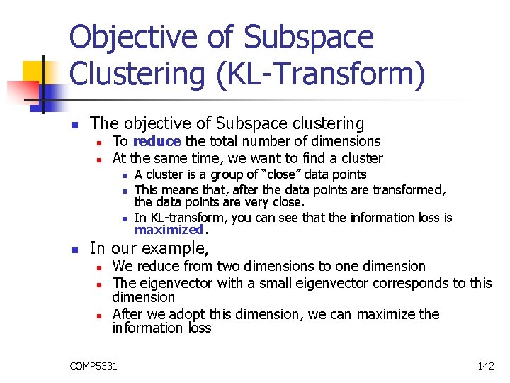
Objective of Subspace Clustering (KL-Transform) n The objective of Subspace clustering n n To reduce the total number of dimensions At the same time, we want to find a cluster n n A cluster is a group of “close” data points This means that, after the data points are transformed, the data points are very close. In KL-transform, you can see that the information loss is maximized. In our example, n n n We reduce from two dimensions to one dimension The eigenvector with a small eigenvector corresponds to this dimension After we adopt this dimension, we can maximize the information loss COMP 5331 142

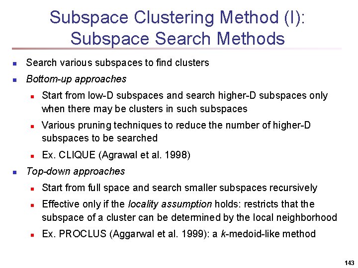
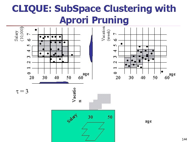
Subspace Clustering Method (I): Subspace Search Methods n Search various subspaces to find clusters n Bottom-up approaches n n Start from low-D subspaces and search higher-D subspaces only when there may be clusters in such subspaces Various pruning techniques to reduce the number of higher-D subspaces to be searched Ex. CLIQUE (Agrawal et al. 1998) Top-down approaches n n n Start from full space and search smaller subspaces recursively Effective only if the locality assumption holds: restricts that the subspace of a cluster can be determined by the local neighborhood Ex. PROCLUS (Aggarwal et al. 1999): a k-medoid-like method 143

=3 30 40 50 20 30 40 50 age 60 Vacatio n 20 age 60 0 1 2 3 4 5 6 7 Vacation (week) 0 1 2 3 4 5 6 7 Salary (10, 000) CLIQUE: Sub. Space Clustering with Aprori Pruning Sa ry a l 30 50 age 144

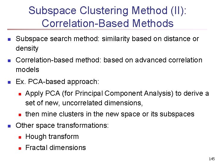
Subspace Clustering Method (II): Correlation-Based Methods n n n Subspace search method: similarity based on distance or density Correlation-based method: based on advanced correlation models Ex. PCA-based approach: n n n Apply PCA (for Principal Component Analysis) to derive a set of new, uncorrelated dimensions, then mine clusters in the new space or its subspaces Other space transformations: n Hough transform n Fractal dimensions 145

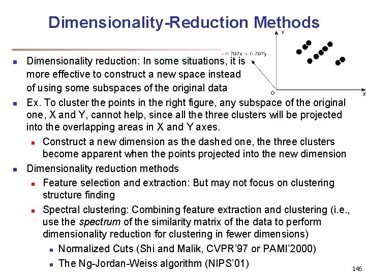
Dimensionality-Reduction Methods n n n Dimensionality reduction: In some situations, it is more effective to construct a new space instead of using some subspaces of the original data Ex. To cluster the points in the right figure, any subspace of the original one, X and Y, cannot help, since all the three clusters will be projected into the overlapping areas in X and Y axes. n Construct a new dimension as the dashed one, the three clusters become apparent when the points projected into the new dimension Dimensionality reduction methods n Feature selection and extraction: But may not focus on clustering structure finding n Spectral clustering: Combining feature extraction and clustering (i. e. , use the spectrum of the similarity matrix of the data to perform dimensionality reduction for clustering in fewer dimensions) n Normalized Cuts (Shi and Malik, CVPR’ 97 or PAMI’ 2000) n The Ng-Jordan-Weiss algorithm (NIPS’ 01) 146

Chapter 11. Cluster Analysis: Advanced Methods n Probability Model-Based Clustering n Clustering High-Dimensional Data n Summary 147

Summary n n Probability Model-Based Clustering n Fuzzy clustering n Probability-model-based clustering n The EM algorithm Clustering High-Dimensional Data n Subspace clustering n Dimensionality reduction 148

References (I) n n n n K. Beyer, J. Goldstein, R. Ramakrishnan, U. Shaft, "When is Nearest Neighbor Meaningful? ", ICDT 1999 R. Agrawal, J. Gehrke, D. Gunopulos, P Raghavan, "Automatic Subspace Clustering of High Dimensional Data for Data Mining Applications", SIGMOD 1998 C. -H. Cheng, A. W. -C. Fu and Y. Zhang, "Entropy-based Subspace Clustering for Mining Numerical Data", SIGKDD 1999 R. Agrawal, J. Gehrke, D. Gunopulos, and P. Raghavan. Automatic subspace clustering of high dimensional data for data mining applications. SIGMOD’ 98 C. C. Aggarwal, C. Procopiuc, J. Wolf, P. S. Yu, and J. -S. Park. Fast algorithms for projected clustering. SIGMOD’ 99 S. Arora, S. Rao, and U. Vazirani. Expander flows, geometric embeddings and graph partitioning. J. ACM, 56: 5: 1– 5: 37, 2009. J. C. Bezdek. Pattern Recognition with Fuzzy Objective Function Algorithms. Plenum Press, 1981. K. S. Beyer, J. Goldstein, R. Ramakrishnan, and U. Shaft. When is ”nearest neighbor” meaningful? ICDT’ 99 Y. Cheng and G. Church. Biclustering of expression data. ISMB’ 00 I. Davidson and S. S. Ravi. Clustering with constraints: Feasibility issues and the k-means algorithm. SDM’ 05 I. Davidson, K. L. Wagstaff, and S. Basu. Measuring constraint-set utility for partitional clustering algorithms. PKDD’ 06 C. Fraley and A. E. Raftery. Model-based clustering, discriminant analysis, and density estimation. J. American Stat. Assoc. , 97: 611– 631, 2002. F. H¨oppner, F. Klawonn, R. Kruse, and T. Runkler. Fuzzy Cluster Analysis: Methods for Classification, Data Analysis and Image Recognition. Wiley, 1999. G. Jeh and J. Widom. Sim. Rank: a measure of structural-context similarity. KDD’ 02 149

References (II) n n n n G. J. Mc. Lachlan and K. E. Bkasford. Mixture Models: Inference and Applications to Clustering. John Wiley & Sons, 1988. B. Mirkin. Mathematical classification and clustering. J. of Global Optimization, 12: 105– 108, 1998. S. C. Madeira and A. L. Oliveira. Biclustering algorithms for biological data analysis: A survey. IEEE/ACM Trans. Comput. Biol. Bioinformatics, 1, 2004. A. Y. Ng, M. I. Jordan, and Y. Weiss. On spectral clustering: Analysis and an algorithm. NIPS’ 01 J. Pei, X. Zhang, M. Cho, H. Wang, and P. S. Yu. Maple: A fast algorithm for maximal pattern-based clustering. ICDM’ 03 M. Radovanovi´c, A. Nanopoulos, and M. Ivanovi´c. Nearest neighbors in high-dimensional data: the emergence and influence of hubs. ICML’ 09 S. E. Schaeffer. Graph clustering. Computer Science Review, 1: 27– 64, 2007. A. K. H. Tung, J. Hou, and J. Han. Spatial clustering in the presence of obstacles. ICDE’ 01 A. K. H. Tung, J. Han, L. V. S. Lakshmanan, and R. T. Ng. Constraint-based clustering in large databases. ICDT’ 01 A. Tanay, R. Sharan, and R. Shamir. Biclustering algorithms: A survey. In Handbook of Computational Molecular Biology, Chapman & Hall, 2004. K. Wagstaff, C. Cardie, S. Rogers, and S. Schr¨odl. Constrained k-means clustering with background knowledge. ICML’ 01 H. Wang, W. Wang, J. Yang, and P. S. Yu. Clustering by pattern similarity in large data sets. SIGMOD’ 02 X. Xu, N. Yuruk, Z. Feng, and T. A. J. Schweiger. SCAN: A structural clustering algorithm for networks. KDD’ 07 X. Yin, J. Han, and P. S. Yu, “Cross-Relational Clustering with User's Guidance”, KDD'05