Mining Frequent Patterns Associations and Correlations Chapter 5
- Slides: 63

Mining Frequent Patterns, Associations, and Correlations (Chapter 5) 2021/6/4 Data Mining: Concepts and Techniques 1

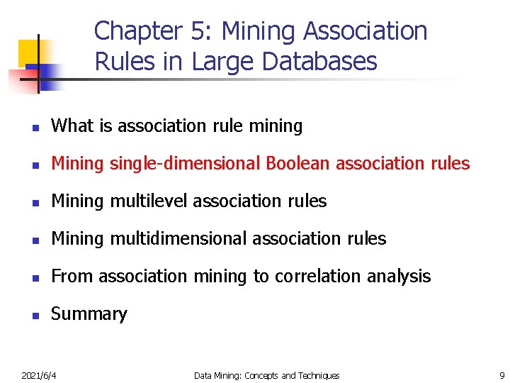
Chapter 5 Mining Frequent Patterns, Associations, and Correlations n What is association rule mining n Mining single-dimensional Boolean association rules n Mining multilevel association rules n Mining multidimensional association rules n From association mining to correlation analysis n Summary 2021/6/4 Data Mining: Concepts and Techniques 2

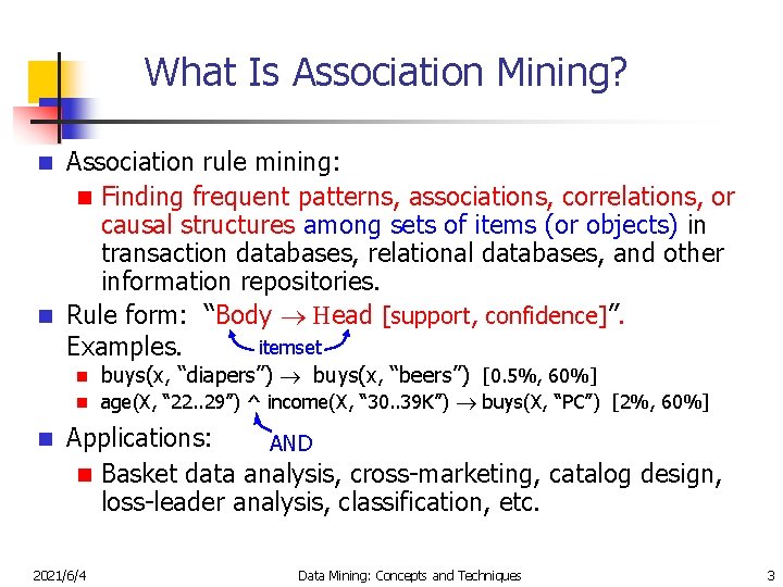
What Is Association Mining? Association rule mining: n Finding frequent patterns, associations, correlations, or causal structures among sets of items (or objects) in transaction databases, relational databases, and other information repositories. n Rule form: “Body ® Head [support, confidence]”. itemset Examples. n n buys(x, “diapers”) ® buys(x, “beers”) [0. 5%, 60%] age(X, “ 22. . 29”) ^ income(X, “ 30. . 39 K”) ® buys(X, “PC”) [2%, 60%] Applications: AND n Basket data analysis, cross-marketing, catalog design, loss-leader analysis, classification, etc. 2021/6/4 Data Mining: Concepts and Techniques 3

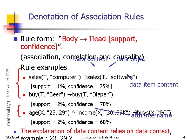
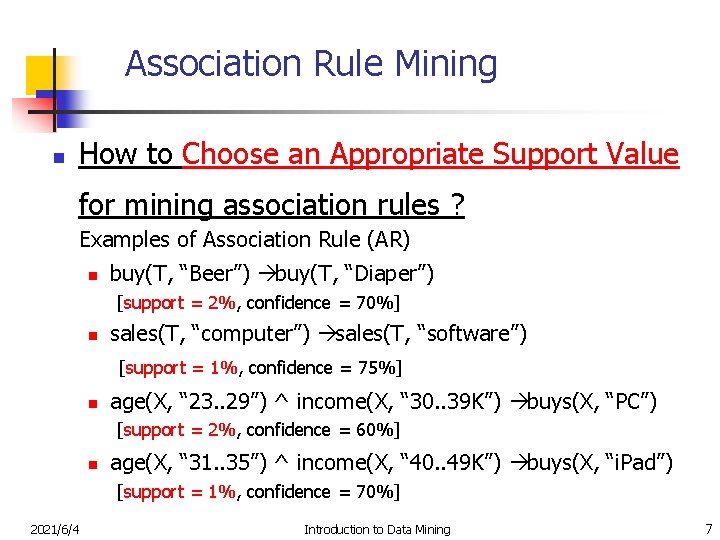
Denotation of Association Rules relational D/B transaction D/B n Rule form: “Body ® Head [support, confidence]”. (association, correlation and causality) data context data object Rule examples n sales(T, “computer”) àsales(T, “software”) [support = 1%, confidence = 75%] n data item content buy(T, “Beer”) àbuy(T, “Diaper”) [support = 2%, confidence = 70%] n age(X, “ 23. . 29”) ^ income(X, “ 30. . 39 K”) àbuys(X, “PC”) attribute name [support = 2%, confidence = 60%] n 2021/6/4 The explanation of data content relies on data context, Introduction to Data Mining 4

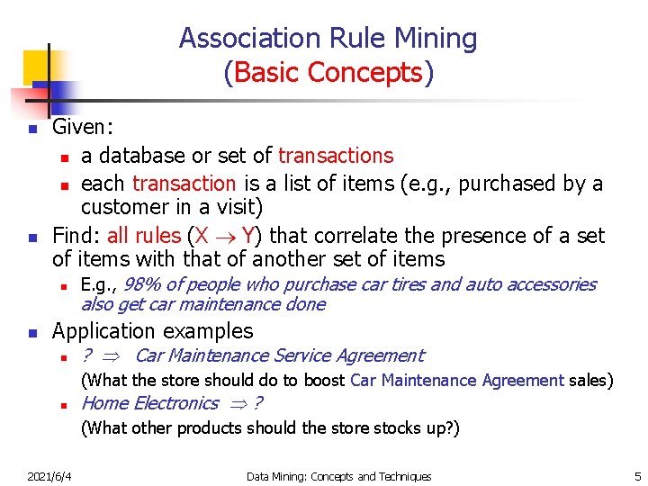
Association Rule Mining (Basic Concepts) n n Given: n a database or set of transactions n each transaction is a list of items (e. g. , purchased by a customer in a visit) Find: all rules (X ® Y) that correlate the presence of a set of items with that of another set of items n n E. g. , 98% of people who purchase car tires and auto accessories also get car maintenance done Application examples n ? Car Maintenance Service Agreement (What the store should do to boost Car Maintenance Agreement sales) n Home Electronics ? (What other products should the store stocks up? ) 2021/6/4 Data Mining: Concepts and Techniques 5

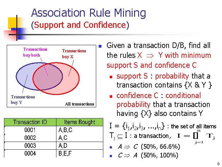
Association Rule Mining (Support and Confidence) Transactions buy both Transactions buy Y Transactions buy X All transactions n Given a transaction D/B, find all the rules X Y with minimum support S and confidence C n support S : probability that a transaction contains {X & Y } n confidence C : conditional probability that a transaction having {X} also contains Y I = {i 1, i 2, i 3, . . . , in} : the set of all items Tj I : a transaction, n n A C (50%, 66. 6%) C A (50%, 100%) 6

Association Rule Mining n How to Choose an Appropriate Support Value for mining association rules ? Examples of Association Rule (AR) n buy(T, “Beer”) àbuy(T, “Diaper”) [support = 2%, confidence = 70%] n sales(T, “computer”) àsales(T, “software”) [support = 1%, confidence = 75%] n age(X, “ 23. . 29”) ^ income(X, “ 30. . 39 K”) àbuys(X, “PC”) [support = 2%, confidence = 60%] n age(X, “ 31. . 35”) ^ income(X, “ 40. . 49 K”) àbuys(X, “i. Pad”) [support = 1%, confidence = 70%] 2021/6/4 Introduction to Data Mining 7

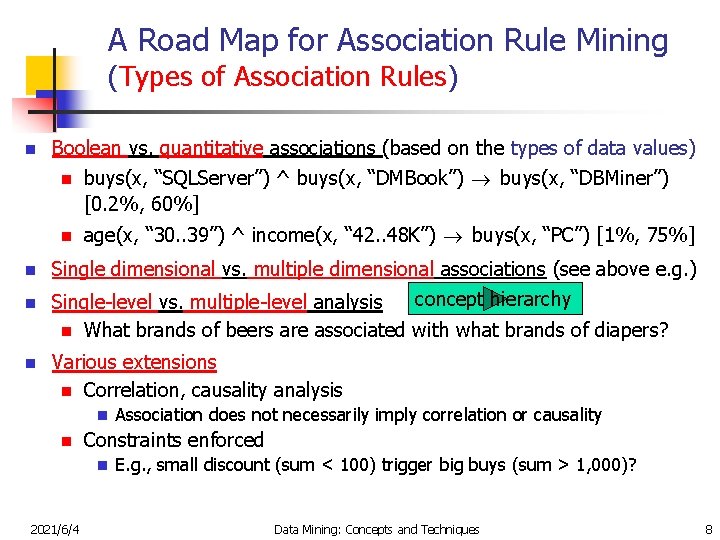
A Road Map for Association Rule Mining (Types of Association Rules) n n Boolean vs. quantitative associations (based on the types of data values) n buys(x, “SQLServer”) ^ buys(x, “DMBook”) ® buys(x, “DBMiner”) [0. 2%, 60%] n age(x, “ 30. . 39”) ^ income(x, “ 42. . 48 K”) ® buys(x, “PC”) [1%, 75%] Single dimensional vs. multiple dimensional associations (see above e. g. ) concept hierarchy Single-level vs. multiple-level analysis n What brands of beers are associated with what brands of diapers? Various extensions n Correlation, causality analysis n n Constraints enforced n 2021/6/4 Association does not necessarily imply correlation or causality E. g. , small discount (sum < 100) trigger big buys (sum > 1, 000)? Data Mining: Concepts and Techniques 8

Chapter 5: Mining Association Rules in Large Databases n What is association rule mining n Mining single-dimensional Boolean association rules n Mining multilevel association rules n Mining multidimensional association rules n From association mining to correlation analysis n Summary 2021/6/4 Data Mining: Concepts and Techniques 9

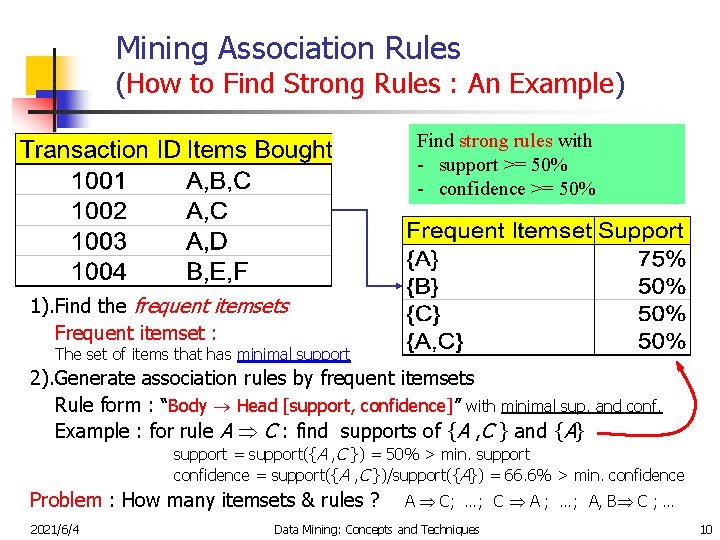
Mining Association Rules (How to Find Strong Rules : An Example) Find strong rules with - support >= 50% - confidence >= 50% 1). Find the frequent itemsets Frequent itemset : The set of items that has minimal support 2). Generate association rules by frequent itemsets Rule form : “Body ® Head [support, confidence]” with minimal sup. and conf. Example : for rule A C : find supports of {A , C } and {A} support = support({A , C }) = 50% > min. support confidence = support({A , C })/support({A}) = 66. 6% > min. confidence Problem : How many itemsets & rules ? 2021/6/4 A C; …; C A ; …; A, B C ; … Data Mining: Concepts and Techniques 10

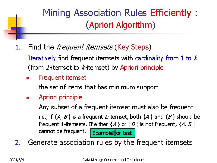
Mining Association Rules Efficiently : (Apriori Algorithm) 1. Find the frequent itemsets (Key Steps) Iteratively find frequent itemsets with cardinality from 1 to k (from 1 -itemset to k-itemset) by Apriori principle n Frequent itemset the set of items that has minimum support n Apriori principle Any subset of a frequent itemset must also be frequent i. e. , if {A, B } is a frequent 2 -itemset, both {A } and {B } should be frequent 1 -itemsets. If either {A } or {B } is not frequent, {A, B } cannot be frequent. Example for test 2. 2021/6/4 Generate association rules by the frequent itemsets Data Mining: Concepts and Techniques 11

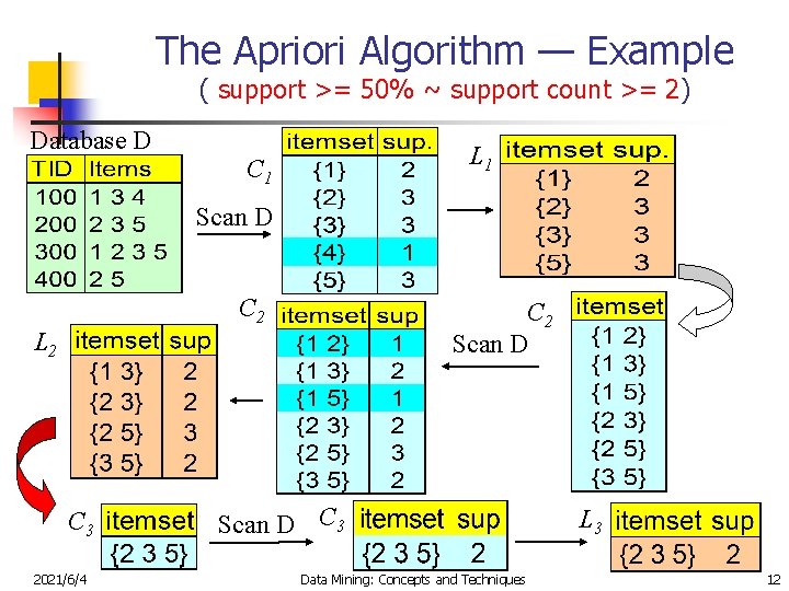
The Apriori Algorithm — Example ( support >= 50% ~ support count >= 2) Database D L 1 C 1 Scan D C 2 Scan D L 2 C 3 2021/6/4 Scan D C 3 Data Mining: Concepts and Techniques L 3 12

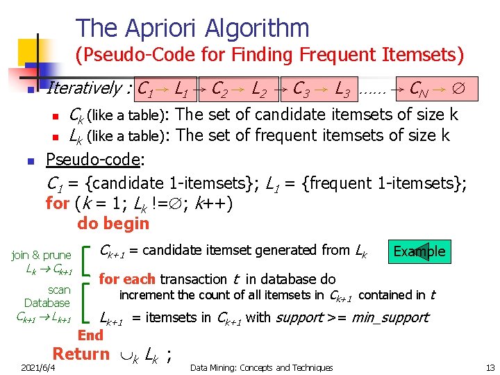
The Apriori Algorithm (Pseudo-Code for Finding Frequent Itemsets) n n Iteratively : C 1 → L 1 → C 2 → L 2 → C 3 → L 3 …… → CN → n Ck (like a table): The set of candidate itemsets of size k n Lk (like a table): The set of frequent itemsets of size k Pseudo-code: C 1 = {candidate 1 -itemsets}; L 1 = {frequent 1 -itemsets}; for (k = 1; Lk != ; k++) do begin join & prune Lk Ck+1 scan Database Ck+1 Lk+1 Ck+1 = candidate itemset generated from Lk Example for each transaction t in database do increment the count of all itemsets in Ck+1 contained in t Lk+1 = itemsets in Ck+1 with support >= min_support End Return k Lk ; 2021/6/4 Data Mining: Concepts and Techniques 13

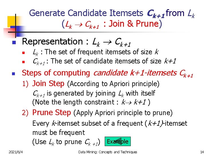
Generate Candidate Itemsets Ck+1 from Lk (Lk Ck+1 : Join & Prune) n Representation : Lk Ck+1 n n n Lk : The set of frequent itemsets of size k Ck+1 : The set of candidate itemsets of size k+1 Steps of computing candidate k+1 -itemsets Ck+1 1) Join Step (According to Apriori principle) Ck+1 is generated by joining Lk with itself (Note the length constraint : k k+1 ) 2) Prune Step (Apply Apriori principle to prune) Every k-itemset subset of a frequent (k+1)-itemset must be frequent (Use Lk to prune Ck +1) Example 2021/6/4 Data Mining: Concepts and Techniques 14

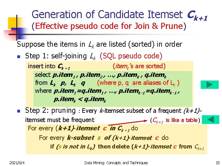
Generation of Candidate Itemset Ck+1 (Effective pseudo code for Join & Prune) Suppose the items in Lk are listed (sorted) in order n Step 1: self-joining Lk (SQL pseudo code) insert into Ck+1 (itemi ’s are sorted) select p. item 1 , p. item 2 , …, p. itemk , q. itemk from Lk p, Lk q (where p, q are aliases of Lk ) where p. item 1=q. item 1 , …, p. itemk-1=q. itemk-1 , p. itemk < q. itemk n Step 2: pruning : Every k-itemset subset of a frequent (k+1)itemset must be frequent For every (k+1)-itemset c in Ck+1 do (Ck+1 is like a table) For every k-subset s of (k+1)-itemset c do if (s is not in Lk) then delete (k+1)-itemset c from Ck+1 2021/6/4 Data Mining: Concepts and Techniques 15

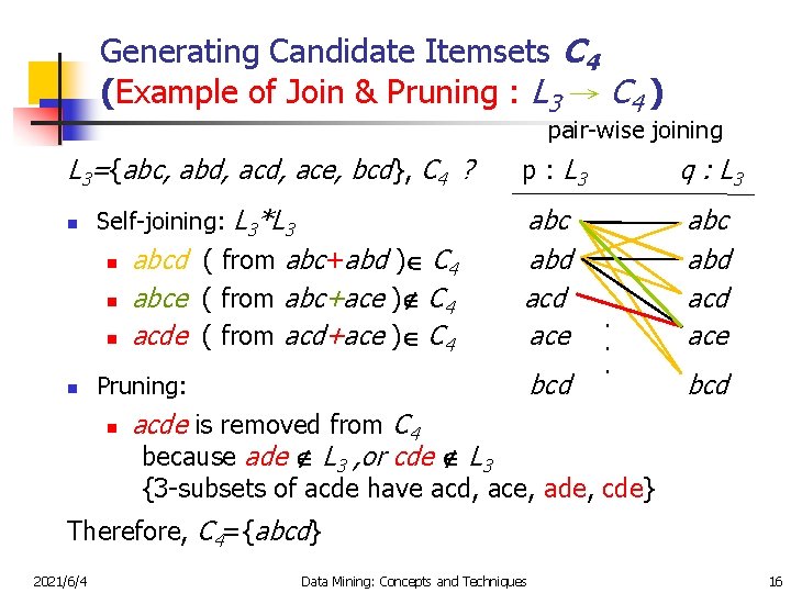
Generating Candidate Itemsets C 4 (Example of Join & Pruning : L 3 → C 4 ) pair-wise joining L 3={abc, abd, ace, bcd}, C 4 ? n Self-joining: L 3*L 3 n n abcd ( from abc+abd ) C 4 abce ( from abc+ace ) C 4 acde ( from acd+ace ) C 4 p : L 3 q : L 3 abc abd acd ace bcd Pruning: n . . . bcd acde is removed from C 4 because ade L 3 , or cde L 3 {3 -subsets of acde have acd, ace, ade, cde} Therefore, C 4={abcd} 2021/6/4 Data Mining: Concepts and Techniques 16

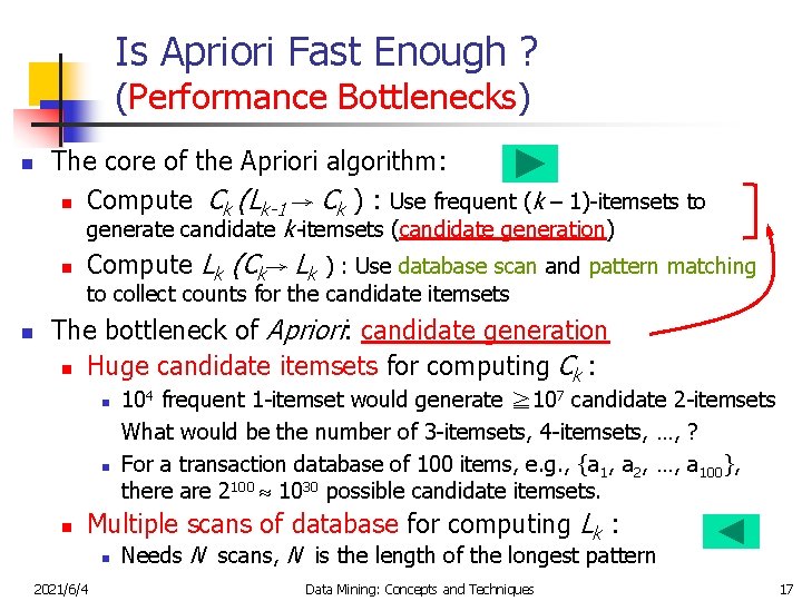
Is Apriori Fast Enough ? (Performance Bottlenecks) n The core of the Apriori algorithm: n Compute Ck (Lk-1 → Ck ) : Use frequent (k – 1)-itemsets to generate candidate k-itemsets (candidate generation) n Compute Lk (Ck→ Lk ) : Use database scan and pattern matching to collect counts for the candidate itemsets n The bottleneck of Apriori: candidate generation n Huge candidate itemsets for computing Ck : n n n 104 frequent 1 -itemset would generate ≧ 107 candidate 2 -itemsets What would be the number of 3 -itemsets, 4 -itemsets, …, ? For a transaction database of 100 items, e. g. , {a 1, a 2, …, a 100}, there are 2100 1030 possible candidate itemsets. Multiple scans of database for computing Lk : n 2021/6/4 Needs N scans, N is the length of the longest pattern Data Mining: Concepts and Techniques 17

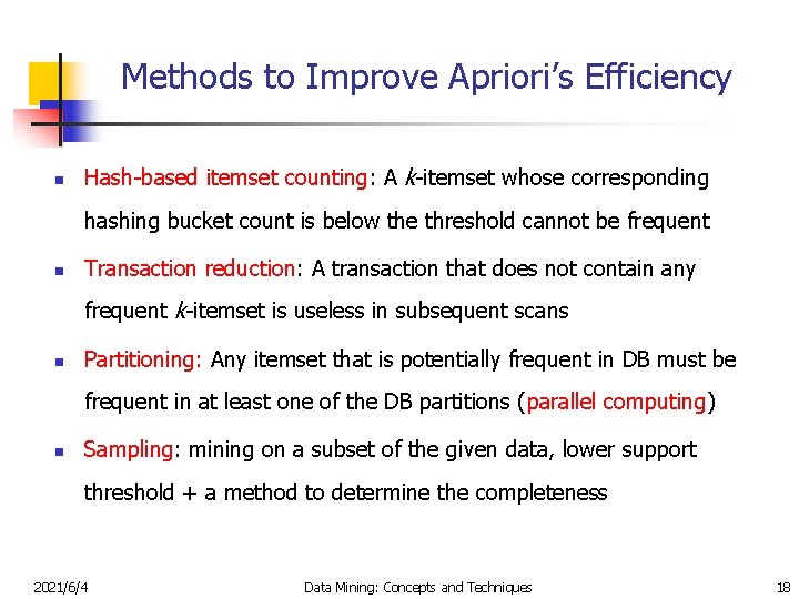
Methods to Improve Apriori’s Efficiency n Hash-based itemset counting: A k-itemset whose corresponding hashing bucket count is below the threshold cannot be frequent n Transaction reduction: A transaction that does not contain any frequent k-itemset is useless in subsequent scans n Partitioning: Any itemset that is potentially frequent in DB must be frequent in at least one of the DB partitions (parallel computing) n Sampling: mining on a subset of the given data, lower support threshold + a method to determine the completeness 2021/6/4 Data Mining: Concepts and Techniques 18

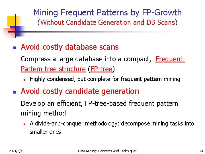
Mining Frequent Patterns by FP-Growth (Without Candidate Generation and DB Scans) n Avoid costly database scans Compress a large database into a compact, Frequent. Pattern tree structure (FP-tree) n n Highly condensed, but complete for frequent pattern mining Avoid costly candidate generation Develop an efficient, FP-tree-based frequent pattern mining method n 2021/6/4 A divide-and-conquer methodology: decompose mining tasks into smaller ones Data Mining: Concepts and Techniques 19

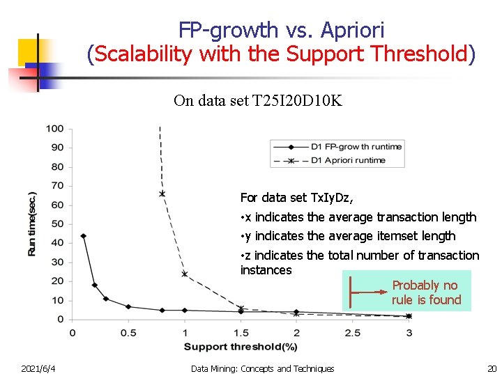
FP-growth vs. Apriori (Scalability with the Support Threshold) On data set T 25 I 20 D 10 K For data set Tx. Iy. Dz, • x indicates the average transaction length • y indicates the average itemset length • z indicates the total number of transaction instances Probably no rule is found 2021/6/4 Data Mining: Concepts and Techniques 20

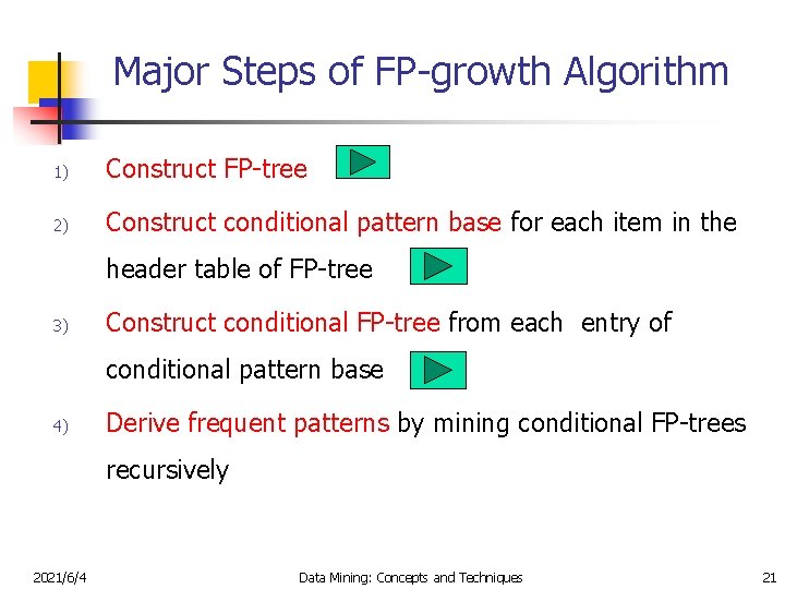
Major Steps of FP-growth Algorithm 1) Construct FP-tree 2) Construct conditional pattern base for each item in the header table of FP-tree 3) Construct conditional FP-tree from each entry of conditional pattern base 4) Derive frequent patterns by mining conditional FP-trees recursively 2021/6/4 Data Mining: Concepts and Techniques 21

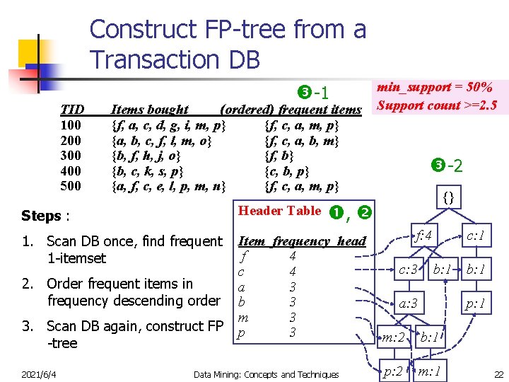
Construct FP-tree from a Transaction DB TID 100 200 300 400 500 -1 Items bought (ordered) frequent items {f, a, c, d, g, i, m, p} {f, c, a, m, p} {a, b, c, f, l, m, o} {f, c, a, b, m} {b, f, h, j, o} {f, b} {b, c, k, s, p} {c, b, p} {a, f, c, e, l, p, m, n} {f, c, a, m, p} Header Table 1. Scan DB once, find frequent 1 -itemset Item frequency head f 4 c 4 a 3 b 3 m 3 p 3 3. Scan DB again, construct FP -tree 2021/6/4 -2 {} , Steps : 2. Order frequent items in frequency descending order min_support = 50% Support count >=2. 5 Data Mining: Concepts and Techniques f: 4 c: 3 c: 1 b: 1 a: 3 b: 1 p: 1 m: 2 b: 1 p: 2 m: 1 22

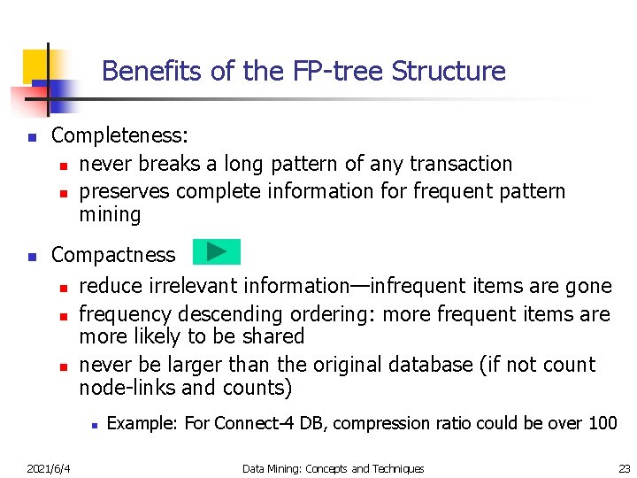
Benefits of the FP-tree Structure n n Completeness: n never breaks a long pattern of any transaction n preserves complete information for frequent pattern mining Compactness n reduce irrelevant information—infrequent items are gone n frequency descending ordering: more frequent items are more likely to be shared n never be larger than the original database (if not count node-links and counts) n 2021/6/4 Example: For Connect-4 DB, compression ratio could be over 100 Data Mining: Concepts and Techniques 23

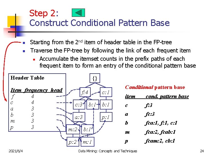
Step 2: Construct Conditional Pattern Base n n Starting from the 2 nd item of header table in the FP-tree Traverse the FP-tree by following the link of each frequent item n Accumulate the itemset counts in the prefix paths of each frequent item to form an entry of the conditional pattern base Header Table Item frequency head f 4 c 4 a 3 b 3 m 3 p 3 2021/6/4 {} f: 4 c: 3 c: 1 b: 1 a: 3 b: 1 p: 1 Conditional pattern base item cond. pattern base c f: 3 a fc: 3 b fca: 1, f: 1, c: 1 m: 2 b: 1 m fca: 2, fcab: 1 p: 2 m: 1 p fcam: 2, cb: 1 Data Mining: Concepts and Techniques 24

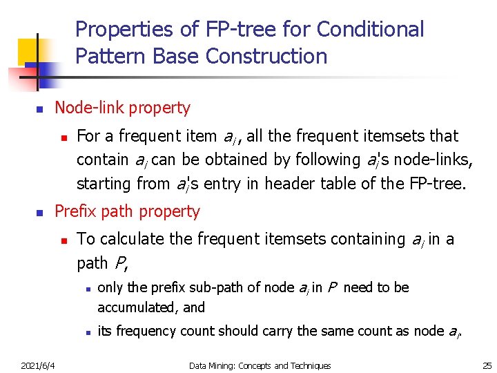
Properties of FP-tree for Conditional Pattern Base Construction n Node-link property n n For a frequent item ai , all the frequent itemsets that contain ai can be obtained by following ai's node-links, starting from ai's entry in header table of the FP-tree. Prefix path property n To calculate the frequent itemsets containing ai in a path P, n n 2021/6/4 only the prefix sub-path of node ai in P need to be accumulated, and its frequency count should carry the same count as node ai. Data Mining: Concepts and Techniques 25

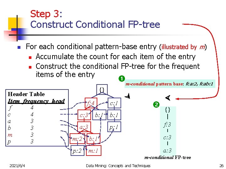
Step 3: Construct Conditional FP-tree n For each conditional pattern-base entry (illustrated by m) n Accumulate the count for each item of the entry n Construct the conditional FP-tree for the frequent items of the entry {} f: 4 c: 3 c: 1 b: 1 a: 3 b: 1 Header Table Item frequency head f 4 c 4 a 3 b 3 m 3 p 3 m-conditional pattern base: fca: 2, fcab: 1 {} f: 3 p: 1 m: 2 b: 1 c: 3 p: 2 m: 1 a: 3 m-conditional FP-tree 2021/6/4 Data Mining: Concepts and Techniques 26

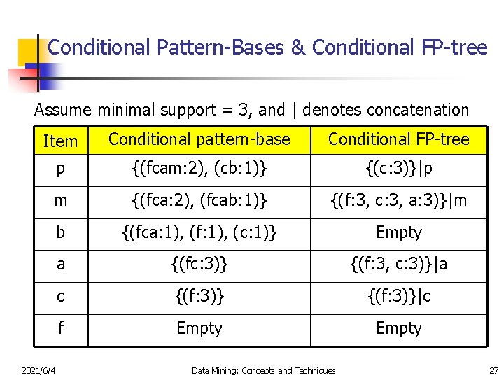
Conditional Pattern-Bases & Conditional FP-tree Assume minimal support = 3, and | denotes concatenation Item Conditional pattern-base Conditional FP-tree p {(fcam: 2), (cb: 1)} {(c: 3)}|p m {(fca: 2), (fcab: 1)} {(f: 3, c: 3, a: 3)}|m b {(fca: 1), (f: 1), (c: 1)} Empty a {(fc: 3)} {(f: 3, c: 3)}|a c {(f: 3)}|c f Empty 2021/6/4 Data Mining: Concepts and Techniques 27

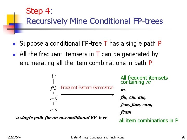
Step 4: Recursively Mine Conditional FP-trees n n Suppose a conditional FP-tree T has a single path P All the frequent itemsets in T can be generated by enumerating all the item combinations in path P {} f: 3 Frequent Pattern Generation c: 3 a single path for an m-conditional FP-tree 2021/6/4 All frequent itemsets containing m m, fm, cm, am, fcm, fam, cam, fcam all item combinations in P Data Mining: Concepts and Techniques 28

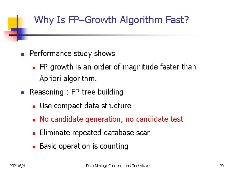
Why Is FP–Growth Algorithm Fast? n Performance study shows n FP-growth is an order of magnitude faster than Apriori algorithm. n 2021/6/4 Reasoning : FP-tree building n Use compact data structure n No candidate generation, no candidate test n Eliminate repeated database scan n Basic operation is counting Data Mining: Concepts and Techniques 29

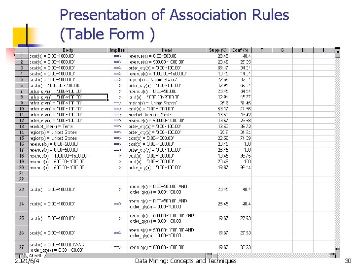
Presentation of Association Rules (Table Form ) 2021/6/4 Data Mining: Concepts and Techniques 30

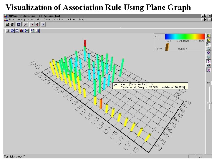
Visualization of Association Rule Using Plane Graph 2021/6/4 Data Mining: Concepts and Techniques 31

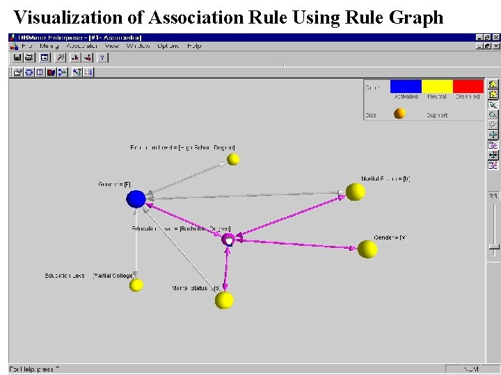
Visualization of Association Rule Using Rule Graph 2021/6/4 Data Mining: Concepts and Techniques 32

Chapter 5: Mining Association Rules in Large Databases n What is association rule mining n Mining single-dimensional Boolean association rules n Mining multilevel association rules n Mining multidimensional association rules n From association mining to correlation analysis n Summary 2021/6/4 Data Mining: Concepts and Techniques 33

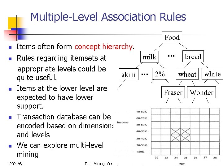
Multiple-Level Association Rules Food n n n Items often form concept hierarchy. … bread milk Rules regarding itemsets at appropriate levels could be … 2% wheat white skim quite useful. Items at the lower level are Fraser Wonder expected to have lower support. Transaction database can be encoded based on dimensions and levels We can explore multi-level mining 2021/6/4 Data Mining: Concepts and Techniques 34

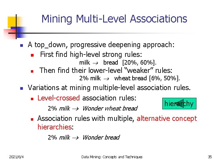
Mining Multi-Level Associations n A top_down, progressive deepening approach: n First find high-level strong rules: milk bread [20%, 60%]. n Then find their lower-level “weaker” rules: 2% milk wheat bread [6%, 50%]. n Variations at mining multiple-level association rules. n Level-crossed association rules: hierarchy 2% milk n Association rules with multiple, alternative concept hierarchies: 2% milk 2021/6/4 Wonder wheat bread Wonder bread Data Mining: Concepts and Techniques 35

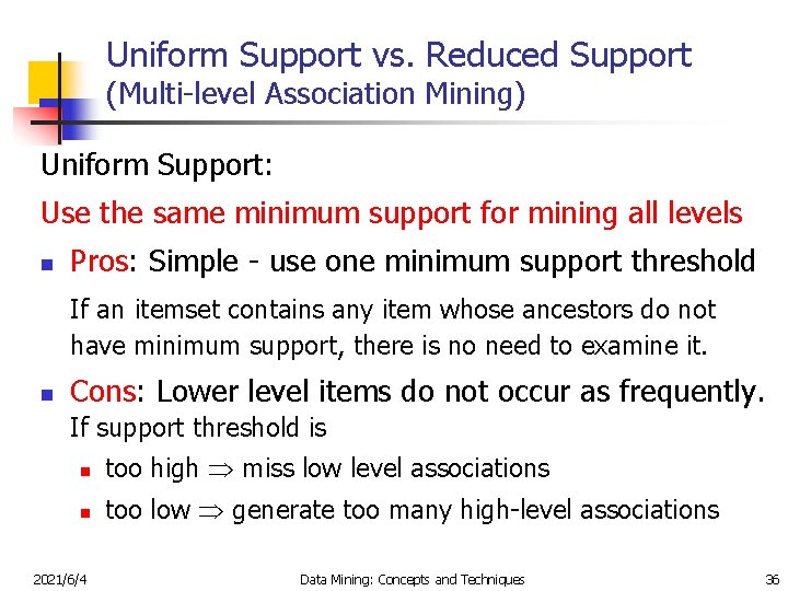
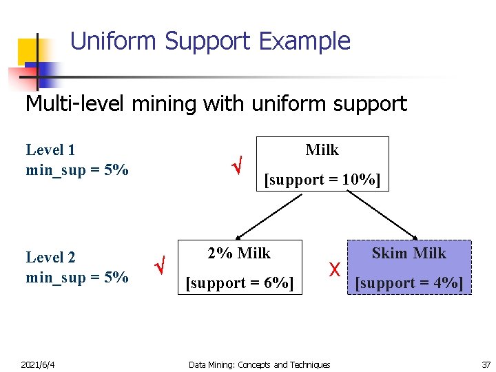
Uniform Support vs. Reduced Support (Multi-level Association Mining) Uniform Support: Use the same minimum support for mining all levels n Pros: Simple - use one minimum support threshold If an itemset contains any item whose ancestors do not have minimum support, there is no need to examine it. n Cons: Lower level items do not occur as frequently. If support threshold is n too high miss low level associations n too low generate too many high-level associations 2021/6/4 Data Mining: Concepts and Techniques 36

Uniform Support Example Multi-level mining with uniform support Level 1 min_sup = 5% Level 2 min_sup = 5% 2021/6/4 Milk [support = 10%] 2% Milk [support = 6%] Χ Data Mining: Concepts and Techniques Skim Milk [support = 4%] 37

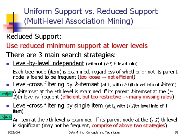
Uniform Support vs. Reduced Support (Multi-level Association Mining) Reduced Support: Use reduced minimum support at lower levels There are 3 main search strategies: n Level-by-level independent (without (i-1)th level info) Each tree node (item) is examined, regardless of whether or not its parent node is found to be frequent (too loose → not efficient) n Example n Level-cross filtering by k-itemset A k-itemset at the i-th level is examined iff its parent k-itemset at the (i 1)th level is frequent (efficient, but too restrictive → many missing rules) Level-cross filtering by single item) Example (at Lk with (i-1)th level info of k-item) (at Lk with (i-1)th level info of 1 - An item at the i-th level is examined iff its parent node at the (i-1)-th level is significant (may not be frequent, comprise of above two strategies) 2021/6/4 Data Mining: Concepts and Techniques 38

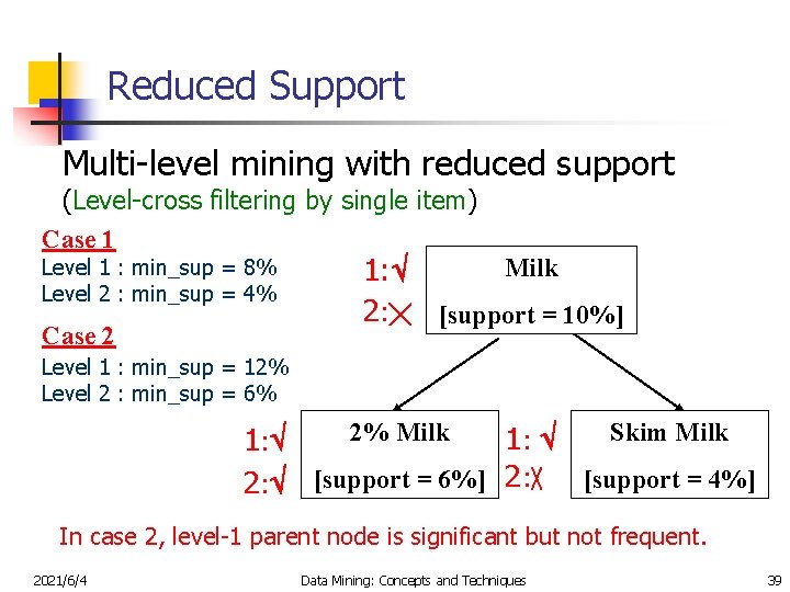
Reduced Support Multi-level mining with reduced support (Level-cross filtering by single item) Case 1 Level 1 : min_sup = 8% Level 2 : min_sup = 4% Case 2 Milk 1: 2: ╳ [support = 10%] Level 1 : min_sup = 12% Level 2 : min_sup = 6% 2% Milk Skim Milk 1: 1 : 2: [support = 6%] 2: ╳ [support = 4%] In case 2, level-1 parent node is significant but not frequent. 2021/6/4 Data Mining: Concepts and Techniques 39

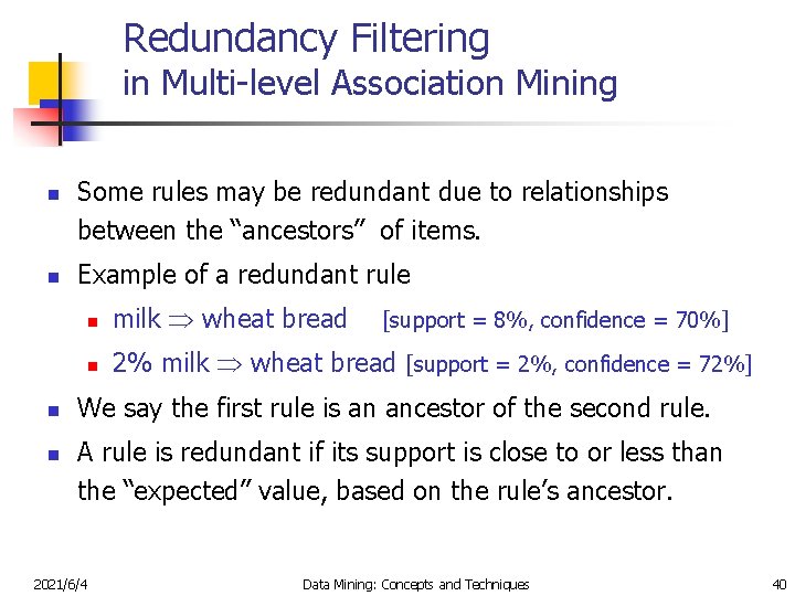
Redundancy Filtering in Multi-level Association Mining n n Some rules may be redundant due to relationships between the “ancestors” of items. Example of a redundant rule n milk wheat bread n 2% milk wheat bread [support = 2%, confidence = 72%] [support = 8%, confidence = 70%] We say the first rule is an ancestor of the second rule. A rule is redundant if its support is close to or less than the “expected” value, based on the rule’s ancestor. 2021/6/4 Data Mining: Concepts and Techniques 40

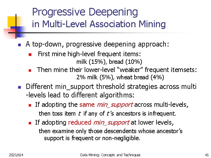
Progressive Deepening in Multi-Level Association Mining n A top-down, progressive deepening approach: n First mine high-level frequent items: milk (15%), bread (10%) n Then mine their lower-level “weaker” frequent itemsets: 2% milk (5%), wheat bread (4%) n Different min_support threshold strategies across multi -levels lead to different algorithms: n If adopting the same min_support across multi-levels, then toss item t if any of t ’s ancestors is infrequent. n If adopting reduced min_support at lower levels, then examine only those descendents whose ancestor’s support is frequent or non-negligible. 2021/6/4 Data Mining: Concepts and Techniques 41

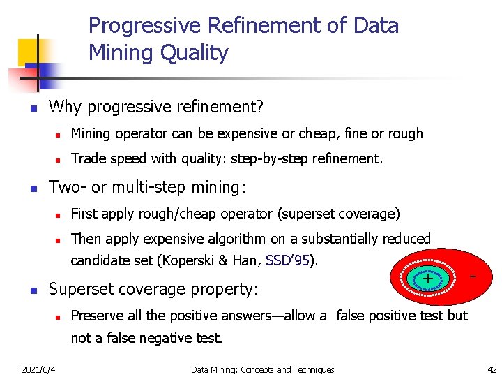
Progressive Refinement of Data Mining Quality n n Why progressive refinement? n Mining operator can be expensive or cheap, fine or rough n Trade speed with quality: step-by-step refinement. Two- or multi-step mining: n First apply rough/cheap operator (superset coverage) n Then apply expensive algorithm on a substantially reduced candidate set (Koperski & Han, SSD’ 95). n Superset coverage property: n + - Preserve all the positive answers—allow a false positive test but not a false negative test. 2021/6/4 Data Mining: Concepts and Techniques 42

Chapter 5: Mining Association Rules in Large Databases n What is association rule mining n Mining single-dimensional Boolean association rules n Mining multilevel association rules n Mining multidimensional association rules n From association mining to correlation analysis n Summary 2021/6/4 Data Mining: Concepts and Techniques 43

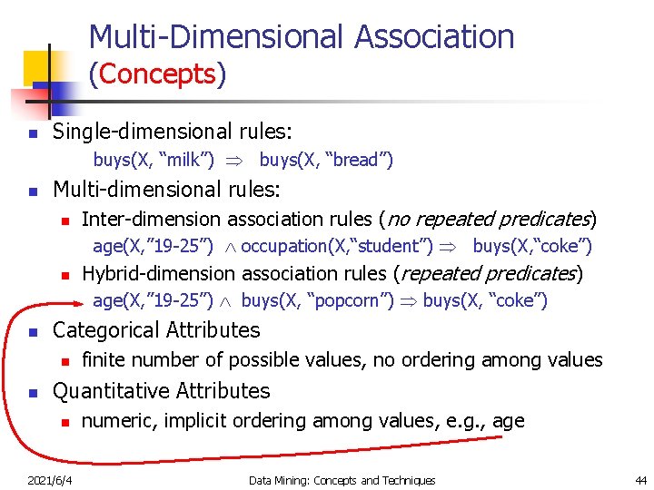
Multi-Dimensional Association (Concepts) n Single-dimensional rules: buys(X, “milk”) buys(X, “bread”) n Multi-dimensional rules: n Inter-dimension association rules (no repeated predicates) age(X, ” 19 -25”) occupation(X, “student”) buys(X, “coke”) n Hybrid-dimension association rules (repeated predicates) age(X, ” 19 -25”) buys(X, “popcorn”) buys(X, “coke”) n Categorical Attributes n n finite number of possible values, no ordering among values Quantitative Attributes n 2021/6/4 numeric, implicit ordering among values, e. g. , age Data Mining: Concepts and Techniques 44

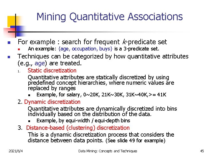
Mining Quantitative Associations n For example : search for frequent k-predicate set n n An example: {age, occupation, buys} is a 3 -predicate set. Techniques can be categorized by how quantitative attributes (e. g. , age) are treated. 1. Static discretization Quantitative attributes are statically discretized by using predefined concept hierarchies, where numeric values are replaced by ranges n Example, for salary, 0~20 K, 21 K~30 K, 31 K~40 K, >= 41 K 2. Dynamic discretization Quantitative attributes are dynamically discretized into bins individually based on the distribution of the data. n Example, by equi-width / equi-depth bins 3. Distance-based (clustering) discretization This is a dynamic discretization process that considers the distance between data points. (See slide 49 for example) 2021/6/4 Data Mining: Concepts and Techniques 45

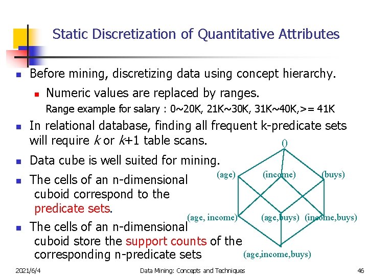
Static Discretization of Quantitative Attributes n Before mining, discretizing data using concept hierarchy. n Numeric values are replaced by ranges. Range example for salary : 0~20 K, 21 K~30 K, 31 K~40 K, >= 41 K n n In relational database, finding all frequent k-predicate sets will require k or k+1 table scans. () Data cube is well suited for mining. (age) (income) (buys) The cells of an n-dimensional cuboid correspond to the predicate sets. (age, income) (age, buys) (income, buys) The cells of an n-dimensional cuboid store the support counts of the (age, income, buys) corresponding n-predicate sets 2021/6/4 Data Mining: Concepts and Techniques 46

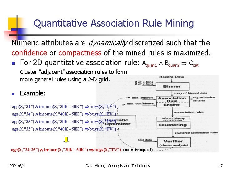
Quantitative Association Rule Mining Numeric attributes are dynamically discretized such that the confidence or compactness of the mined rules is maximized. n For 2 D quantitative association rule: Aquan 1 Bquan 2 Ccat Cluster “adjacent” association rules to form more general rules using a 2 -D grid. n Example: age(X, ” 34”) income(X, ” 30 K - 40 K”) buys(X, ”TV”) age(X, ” 34”) income(X, ” 40 K - 50 K”) buys(X, ”TV”) age(X, ” 35”) income(X, ” 30 K - 40 K”) buys(X, ”TV”) age(X, ” 35”) income(X, ” 40 K - 50 K”) buys(X, ”TV”) age(X, ” 34 -35”) income(X, ” 30 K - 50 K”) buys(X, ”TV”) (more compact) 2021/6/4 Data Mining: Concepts and Techniques 47

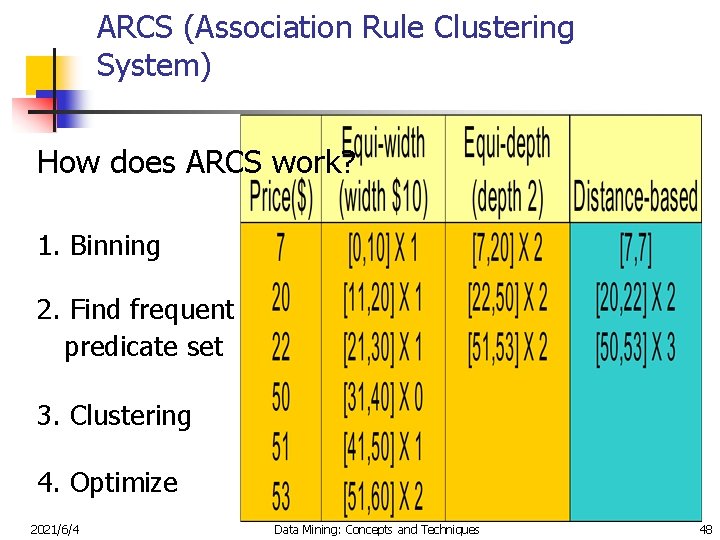
ARCS (Association Rule Clustering System) How does ARCS work? 1. Binning 2. Find frequent predicate set 3. Clustering 4. Optimize 2021/6/4 Data Mining: Concepts and Techniques 48

Limitations of ARCS n Only quantitative attributes on LHS of rules. n Only 2 attributes on LHS. (2 D limitation) n An alternative to ARCS n Non-grid-based n equi-depth binning n n 2021/6/4 clustering based on a measure of partial completeness. “Mining Quantitative Association Rules in Large Relational Tables” by R. Srikant and R. Agrawal. Data Mining: Concepts and Techniques 49

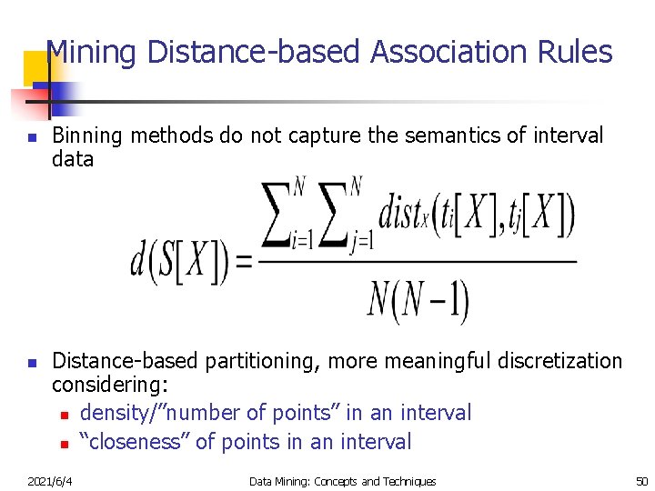
Mining Distance-based Association Rules n n Binning methods do not capture the semantics of interval data Distance-based partitioning, more meaningful discretization considering: n density/”number of points” in an interval n “closeness” of points in an interval 2021/6/4 Data Mining: Concepts and Techniques 50

Chapter 5: Mining Association Rules in Large Databases n What is association rule mining n Mining single-dimensional Boolean association rules n Mining multilevel association rules n Mining multidimensional association rules n From association mining to correlation analysis n Summary 2021/6/4 Data Mining: Concepts and Techniques 53

Interestingness Measurements of Association Rules n Objective measures Two popular measurements: n n n 2021/6/4 support confidence Subjective measures (Silberschatz & Tuzhilin, KDD 95) A rule (pattern) is interesting if n it is unexpected (surprising to the user); and/or n actionable (the user can do something with it) Data Mining: Concepts and Techniques 54

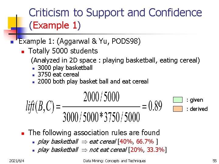
Criticism to Support and Confidence (Example 1) n Example 1: (Aggarwal & Yu, PODS 98) n Totally 5000 students (Analyzed in 2 D space : playing basketball, eating cereal) n n n 3000 play basketball 3750 eat cereal 2000 both play basket ball and eat cereal : given : derived n The following association rules are found n n 2021/6/4 play basketball eat cereal [40%, 66. 7% ] play basketball not eat cereal [20%, 33. 3%] Data Mining: Concepts and Techniques 55

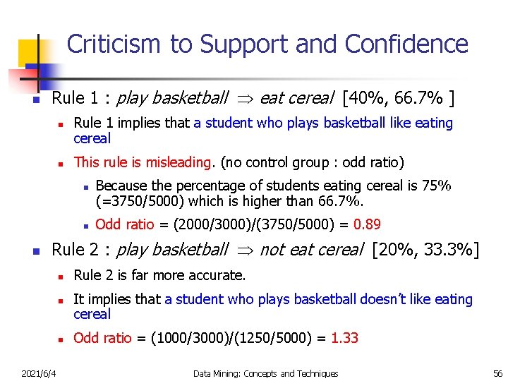
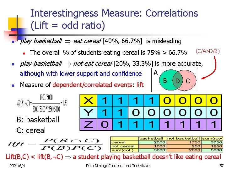
Criticism to Support and Confidence n Rule 1 : play basketball eat cereal [40%, 66. 7% ] n n Rule 1 implies that a student who plays basketball like eating cereal This rule is misleading. (no control group : odd ratio) n n n Because the percentage of students eating cereal is 75% (=3750/5000) which is higher than 66. 7%. Odd ratio = (2000/3000)/(3750/5000) = 0. 89 Rule 2 : play basketball not eat cereal [20%, 33. 3%] n n n 2021/6/4 Rule 2 is far more accurate. It implies that a student who plays basketball doesn’t like eating cereal Odd ratio = (1000/3000)/(1250/5000) = 1. 33 Data Mining: Concepts and Techniques 56

Interestingness Measure: Correlations (Lift = odd ratio) n play basketball eat cereal [40%, 66. 7%] is misleading n n The overall % of students eating cereal is 75% > 66. 7%. play basketball not eat cereal [20%, 33. 3%] is more accurate, although with lower support and confidence n (C/A>D/B) Measure of dependent/correlated events: lift A B D C B: basketball C: cereal Lift(B, C) < lift(B, ¬C) a student playing basketball doesn’t like eating cereal 2021/6/4 Data Mining: Concepts and Techniques 57

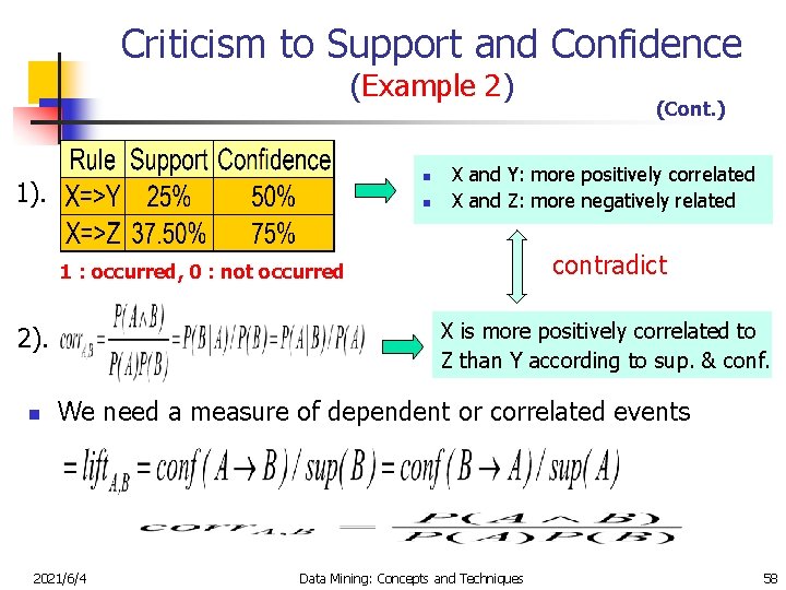
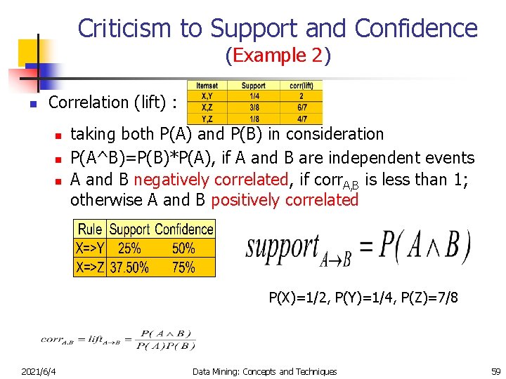
Criticism to Support and Confidence (Example 2) n 1). n X and Y: more positively correlated X and Z: more negatively related contradict 1 : occurred, 0 : not occurred X is more positively correlated to Z than Y according to sup. & conf. 2). n (Cont. ) We need a measure of dependent or correlated events 2021/6/4 Data Mining: Concepts and Techniques 58

Criticism to Support and Confidence (Example 2) n Correlation (lift) : n n n taking both P(A) and P(B) in consideration P(A^B)=P(B)*P(A), if A and B are independent events A and B negatively correlated, if corr. A, B is less than 1; otherwise A and B positively correlated P(X)=1/2, P(Y)=1/4, P(Z)=7/8 2021/6/4 Data Mining: Concepts and Techniques 59

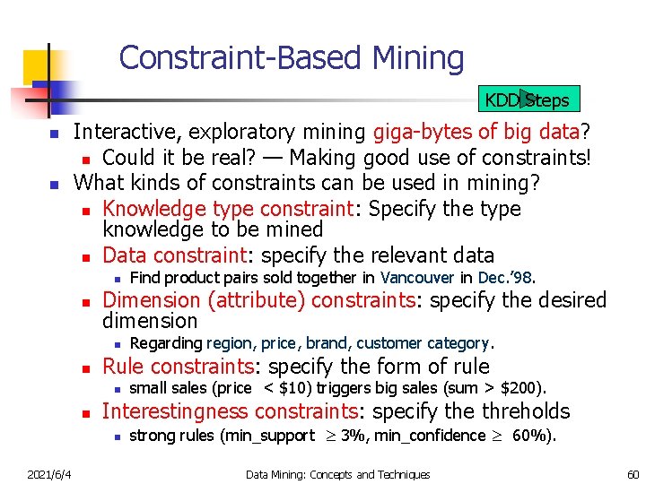
Constraint-Based Mining KDD Steps n n Interactive, exploratory mining giga-bytes of big data? n Could it be real? — Making good use of constraints! What kinds of constraints can be used in mining? n Knowledge type constraint: Specify the type knowledge to be mined n Data constraint: specify the relevant data n n Dimension (attribute) constraints: specify the desired dimension n n small sales (price < $10) triggers big sales (sum > $200). Interestingness constraints: specify the threholds n 2021/6/4 Regarding region, price, brand, customer category. Rule constraints: specify the form of rule n n Find product pairs sold together in Vancouver in Dec. ’ 98. strong rules (min_support 3%, min_confidence 60%). Data Mining: Concepts and Techniques 60

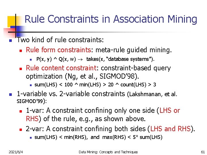
Rule Constraints in Association Mining n Two kind of rule constraints: n Rule form constraints: meta-rule guided mining. n n Rule content constraint: constraint-based query optimization (Ng, et al. , SIGMOD’ 98). n n P(x, y) ^ Q(x, w) ® takes(x, “database systems”). sum(LHS) < 100 ^ min(LHS) > 20 ^ count(LHS) > 3 1 -variable vs. 2 -variable constraints (Lakshmanan, et al. SIGMOD’ 99): n n 1 -var: A constraint confining only one side (LHS or RHS) of the rule, e. g. , as shown above. 2 -var: A constraint confining both sides (LHS and RHS). n 2021/6/4 sum(LHS) < min(RHS), and max(RHS) < 5* sum(LHS) Data Mining: Concepts and Techniques 61

Chapter 5: Mining Association Rules in Large Databases n What is association rule mining n Mining single-dimensional Boolean association rules n Mining multilevel association rules n Mining multidimensional association rules n From association mining to correlation analysis n Summary 2021/6/4 Data Mining: Concepts and Techniques 62

Why Is the Big Pie Still There? n More on constraint-based mining of associations n Boolean vs. quantitative associations n n From association to correlation and causal structure analysis. n n E. g. , break the barriers of transactions (Lu, et al. TOIS’ 99). From association analysis to classification and clustering analysis n 2021/6/4 Association does not necessarily imply correlation or causal relationships From intra-transaction association to inter-transaction associations n n Association on discrete vs. continuous data E. g, clustering association rules Data Mining: Concepts and Techniques 63

Summary n Association rule mining n probably the most significant contribution from the database community in KDD n A large number of papers have been published n Many interesting issues have been explored n An interesting research direction n Association analysis in other types of data: spatial data, multimedia data, time series data, etc. 2021/6/4 Data Mining: Concepts and Techniques 64

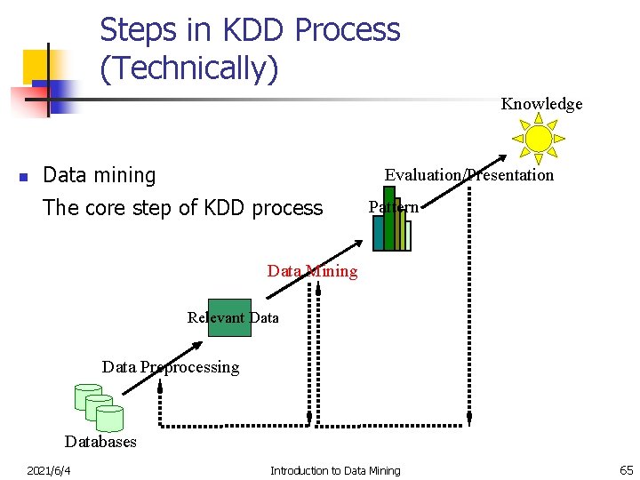
Steps in KDD Process (Technically) Knowledge n Data mining Evaluation/Presentation The core step of KDD process Pattern Data Mining Relevant Data Preprocessing Databases 2021/6/4 Introduction to Data Mining 65