Lecture 2 Data Mining 1 Roadmap What is

Lecture 2: Data Mining 1

Roadmap • What is data mining? • Data Mining Tasks – Classification/Decision Tree – Clustering – Association Mining • Data Mining Algorithms – Decision Tree Construction – Frequent 2 -itemsets – Frequent Itemsets (Apriori) – Clustering/Collaborative Filtering 2

What is Data Mining? • Discovery of useful, possibly unexpected, patterns in data. • Subsidiary issues: – Data cleansing: detection of bogus data. • E. g. , age = 150. – Visualization: something better than megabyte files of output. – Warehousing of data (for retrieval). 3

Typical Kinds of Patterns 1. 2. 3. Decision trees: succinct ways to classify by testing properties. Clusters: another succinct classification by similarity of properties. Bayes, hidden-Markov, and other statistical models, frequentitemsets: expose important associations within data. 4

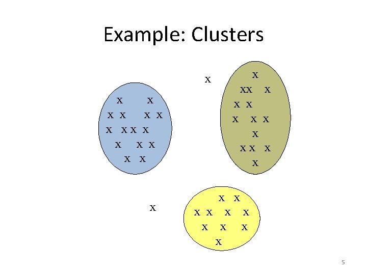
Example: Clusters x x x x xx x x x x x x 5

Applications (Among Many) • Intelligence-gathering. – Total Information Awareness. • Web Analysis. – Page. Rank. • Marketing. – Run a sale on diapers; raise the price of beer. • Detective? 6

Cultures • Databases: concentrate on large-scale (non-main-memory) data. • AI (machine-learning): concentrate on complex methods, small data. • Statistics: concentrate on inferring models. 7

Models vs. Analytic Processing • To a database person, data-mining is a powerful form of analytic processing --- queries that examine large amounts of data. – Result is the data that answers the query. • To a statistician, data-mining is the inference of models. – Result is the parameters of the model. 8

Meaningfulness of Answers • A big risk when data mining is that you will “discover” patterns that are meaningless. • Statisticians call it Bonferroni’s principle: (roughly) if you look in more places for interesting patterns than your amount of data will support, you are bound to find crap. 9

Examples • A big objection to TIA was that it was looking for so many vague connections that it was sure to find things that were bogus and thus violate innocents’ privacy. • The Rhine Paradox: a great example of how not to conduct scientific research. 10

Rhine Paradox --- (1) • David Rhine was a parapsychologist in the 1950’s who hypothesized that some people had Extra-Sensory Perception. • He devised an experiment where subjects were asked to guess 10 hidden cards --- red or blue. • He discovered that almost 1 in 1000 had ESP --- they were able to get all 10 right! 11

Rhine Paradox --- (2) • He told these people they had ESP and called them in for another test of the same type. • Alas, he discovered that almost all of them had lost their ESP. • What did he conclude? – Answer on next slide. 12

Rhine Paradox --- (3) • He concluded that you shouldn’t tell people they have ESP; it causes them to lose it. 13

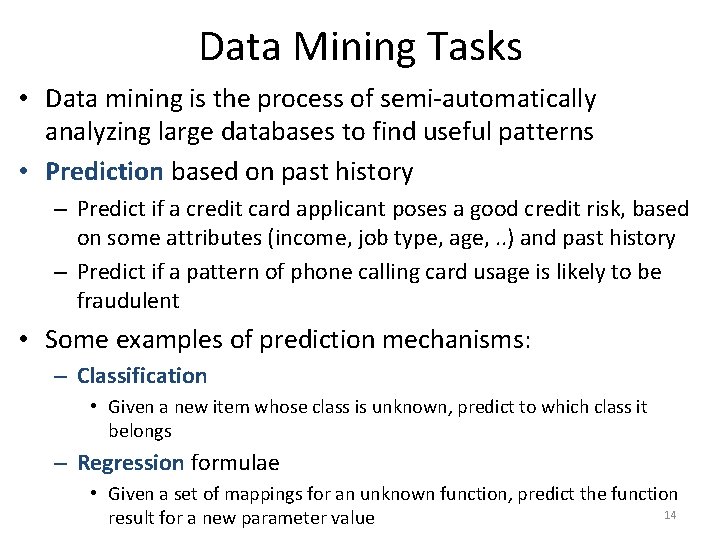
Data Mining Tasks • Data mining is the process of semi-automatically analyzing large databases to find useful patterns • Prediction based on past history – Predict if a credit card applicant poses a good credit risk, based on some attributes (income, job type, age, . . ) and past history – Predict if a pattern of phone calling card usage is likely to be fraudulent • Some examples of prediction mechanisms: – Classification • Given a new item whose class is unknown, predict to which class it belongs – Regression formulae • Given a set of mappings for an unknown function, predict the function 14 result for a new parameter value

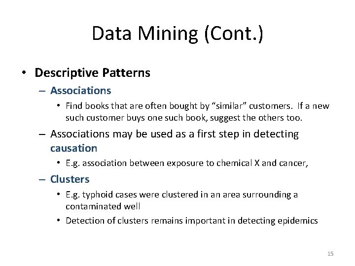
Data Mining (Cont. ) • Descriptive Patterns – Associations • Find books that are often bought by “similar” customers. If a new such customer buys one such book, suggest the others too. – Associations may be used as a first step in detecting causation • E. g. association between exposure to chemical X and cancer, – Clusters • E. g. typhoid cases were clustered in an area surrounding a contaminated well • Detection of clusters remains important in detecting epidemics 15

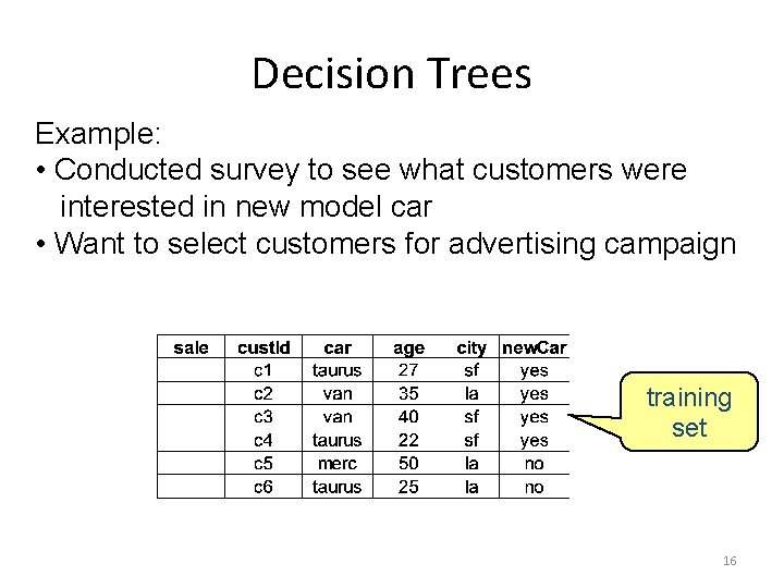
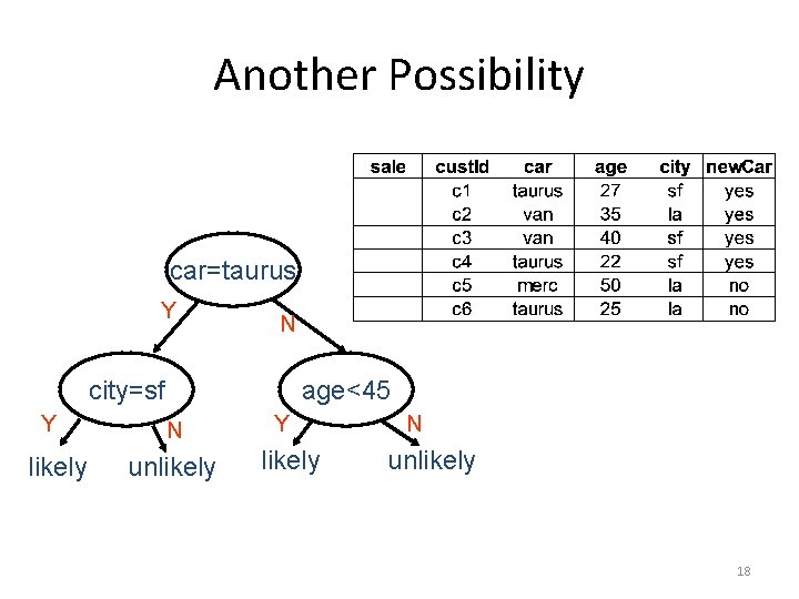
Decision Trees Example: • Conducted survey to see what customers were interested in new model car • Want to select customers for advertising campaign training set 16

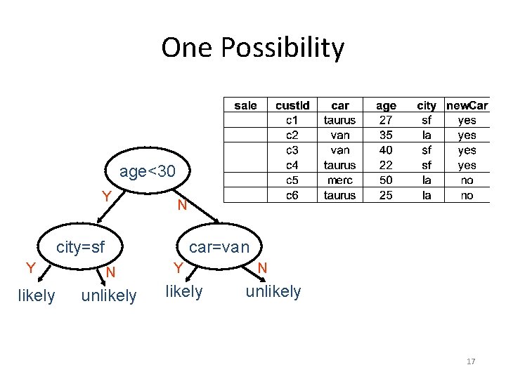
One Possibility age<30 Y N city=sf Y likely car=van N unlikely Y likely N unlikely 17

Another Possibility car=taurus Y N city=sf Y likely age<45 N unlikely Y likely N unlikely 18

Issues • Decision tree cannot be “too deep” • would not have statistically significant amounts of data for lower decisions • Need to select tree that most reliably predicts outcomes 19

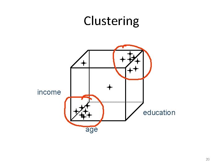
Clustering income education age 20

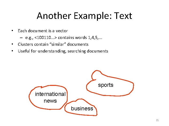
Another Example: Text • Each document is a vector – e. g. , <100110. . . > contains words 1, 4, 5, . . . • Clusters contain “similar” documents • Useful for understanding, searching documents sports international news business 21

Issues • Given desired number of clusters? • Finding “best” clusters • Are clusters semantically meaningful? 22

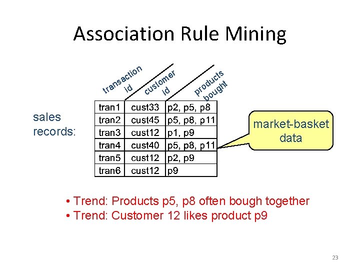
Association Rule Mining n sa tra sales records: on i t c id r e m sto u c id ts c du ht o pr oug b market-basket data • Trend: Products p 5, p 8 often bough together • Trend: Customer 12 likes product p 9 23

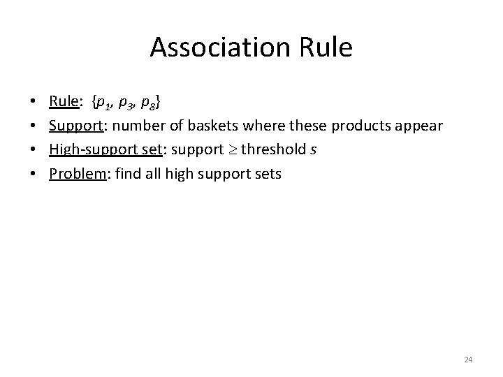
Association Rule • • Rule: {p 1, p 3, p 8} Support: number of baskets where these products appear High-support set: support threshold s Problem: find all high support sets 24

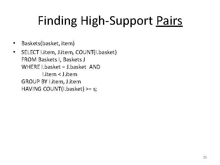
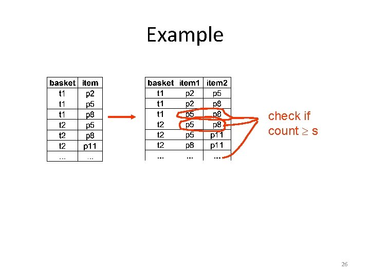
Finding High-Support Pairs • Baskets(basket, item) • SELECT I. item, J. item, COUNT(I. basket) FROM Baskets I, Baskets J WHERE I. basket = J. basket AND I. item < J. item GROUP BY I. item, J. item HAVING COUNT(I. basket) >= s; 25

Example check if count s 26

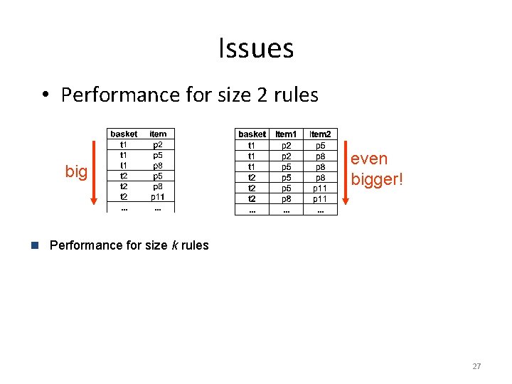
Issues • Performance for size 2 rules big even bigger! n Performance for size k rules 27

Roadmap • What is data mining? • Data Mining Tasks – Classification/Decision Tree – Clustering – Association Mining • Data Mining Algorithms – Decision Tree Construction – Frequent 2 -itemsets – Frequent Itemsets (Apriori) – Clustering/Collaborative Filtering 28

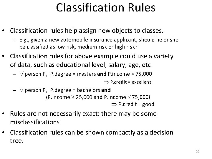
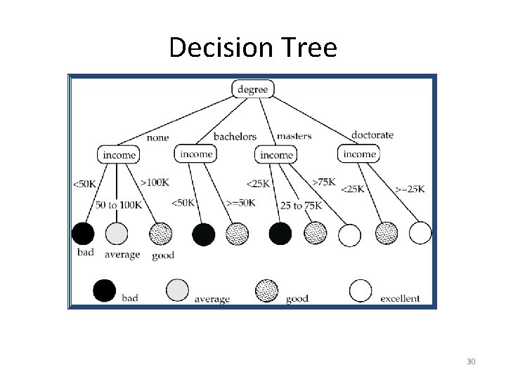
Classification Rules • Classification rules help assign new objects to classes. – E. g. , given a new automobile insurance applicant, should he or she be classified as low risk, medium risk or high risk? • Classification rules for above example could use a variety of data, such as educational level, salary, age, etc. – person P, P. degree = masters and P. income > 75, 000 P. credit = excellent – person P, P. degree = bachelors and (P. income 25, 000 and P. income 75, 000) P. credit = good • Rules are not necessarily exact: there may be some misclassifications • Classification rules can be shown compactly as a decision tree. 29

Decision Tree 30

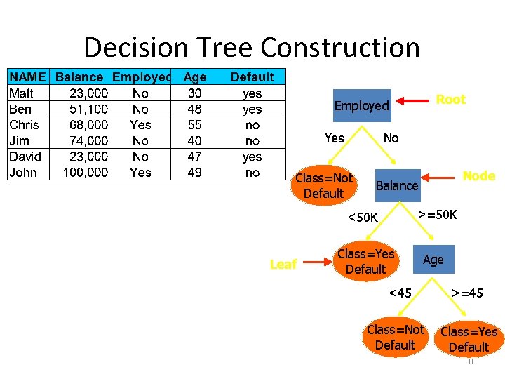
Decision Tree Construction Root Employed Yes No Class=Not Default Leaf Node Balance <50 K >=50 K Class=Yes Default Age <45 Class=Not Default >=45 Class=Yes Default 31

Construction of Decision Trees • Training set: a data sample in which the classification is already known. • Greedy top down generation of decision trees. – Each internal node of the tree partitions the data into groups based on a partitioning attribute, and a partitioning condition for the node – Leaf node: • all (or most) of the items at the node belong to the same class, or • all attributes have been considered, and no further partitioning is possible. 32

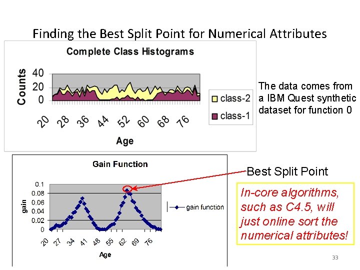
Finding the Best Split Point for Numerical Attributes The data comes from a IBM Quest synthetic dataset for function 0 Best Split Point In-core algorithms, such as C 4. 5, will just online sort the numerical attributes! 33

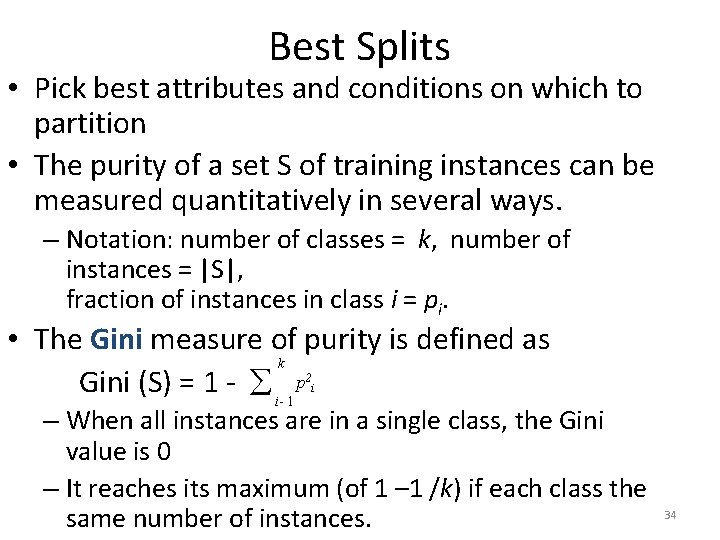
Best Splits • Pick best attributes and conditions on which to partition • The purity of a set S of training instances can be measured quantitatively in several ways. – Notation: number of classes = k, number of instances = |S|, fraction of instances in class i = pi. • The Gini measure of purity is defined as k Gini (S) = 1 - i- 1 p 2 i – When all instances are in a single class, the Gini value is 0 – It reaches its maximum (of 1 – 1 /k) if each class the same number of instances. 34

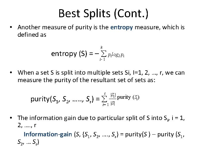
Best Splits (Cont. ) • Another measure of purity is the entropy measure, which is defined as k entropy (S) = – pilog 2 pi i- 1 • When a set S is split into multiple sets Si, I=1, 2, …, r, we can measure the purity of the resultant set of sets as: r purity(S 1, S 2, …. . , Sr) = |Si| i= 1 |S| purity (Si) • The information gain due to particular split of S into Si, i = 1, 2, …. , r Information-gain (S, {S 1, S 2, …. , Sr) = purity(S ) – purity (S 1, S 2 , … Sr )

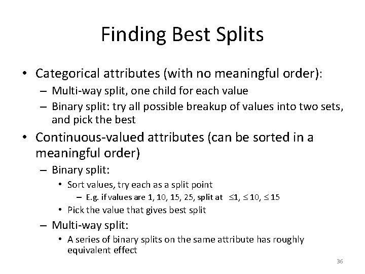
Finding Best Splits • Categorical attributes (with no meaningful order): – Multi-way split, one child for each value – Binary split: try all possible breakup of values into two sets, and pick the best • Continuous-valued attributes (can be sorted in a meaningful order) – Binary split: • Sort values, try each as a split point – E. g. if values are 1, 10, 15, 25, split at 1, 10, 15 • Pick the value that gives best split – Multi-way split: • A series of binary splits on the same attribute has roughly equivalent effect 36

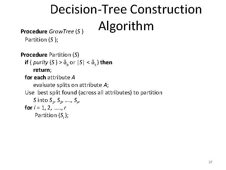
Decision-Tree Construction Algorithm Procedure Grow. Tree (S ) Partition (S ); Procedure Partition (S) if ( purity (S ) > p or |S| < s ) then return; for each attribute A evaluate splits on attribute A; Use best split found (across all attributes) to partition S into S 1, S 2, …. , Sr, for i = 1, 2, …. . , r Partition (Si ); 37

Finding Association Rules • We are generally only interested in association rules with reasonably high support (e. g. support of 2% or greater) • Naïve algorithm 1. Consider all possible sets of relevant items. 2. For each set find its support (i. e. count how many transactions purchase all items in the set). H Large itemsets: sets with sufficiently high support 38

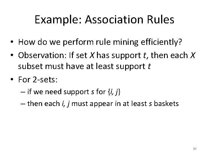
Example: Association Rules • How do we perform rule mining efficiently? • Observation: If set X has support t, then each X subset must have at least support t • For 2 -sets: – if we need support s for {i, j} – then each i, j must appear in at least s baskets 39

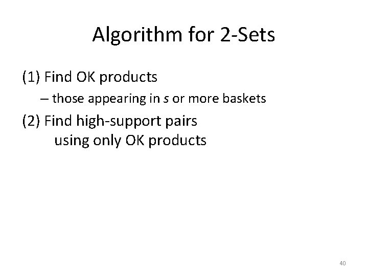
Algorithm for 2 -Sets (1) Find OK products – those appearing in s or more baskets (2) Find high-support pairs using only OK products 40

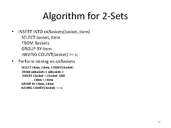
Algorithm for 2 -Sets • INSERT INTO ok. Baskets(basket, item) SELECT basket, item FROM Baskets GROUP BY item HAVING COUNT(basket) >= s; • Perform mining on ok. Baskets SELECT I. item, J. item, COUNT(I. basket) FROM ok. Baskets I, ok. Baskets J WHERE I. basket = J. basket AND I. item < J. item GROUP BY I. item, J. item HAVING COUNT(I. basket) >= s; 41

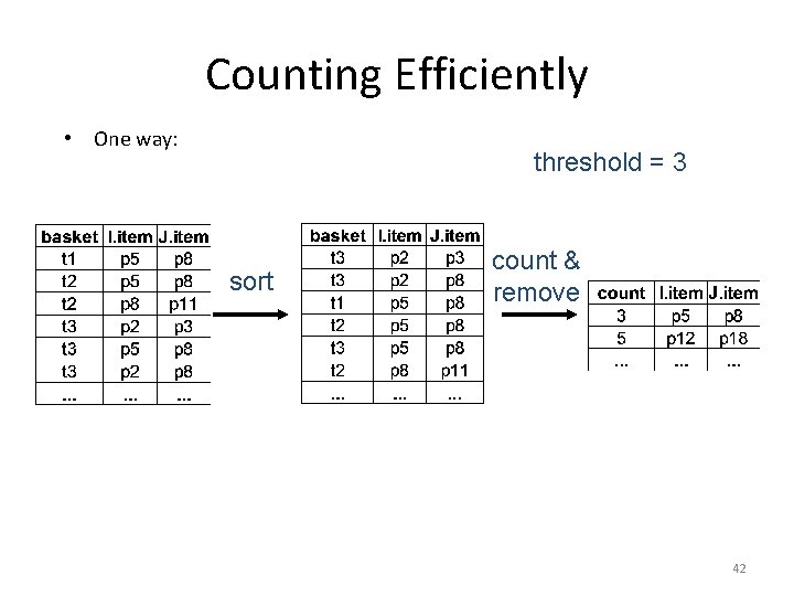
Counting Efficiently • One way: threshold = 3 sort count & remove 42

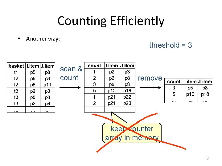
Counting Efficiently • Another way: threshold = 3 scan & count remove keep counter array in memory 43

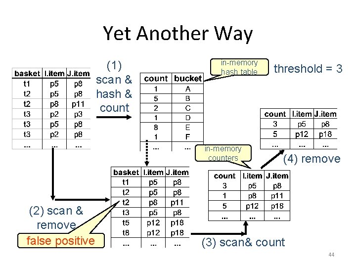
Yet Another Way (1) scan & hash & count in-memory hash table in-memory counters (2) scan & remove false positive threshold = 3 (4) remove (3) scan& count 44

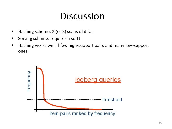
Discussion frequency • Hashing scheme: 2 (or 3) scans of data • Sorting scheme: requires a sort! • Hashing works well if few high-support pairs and many low-support ones iceberg queries threshold item-pairs ranked by frequency 45

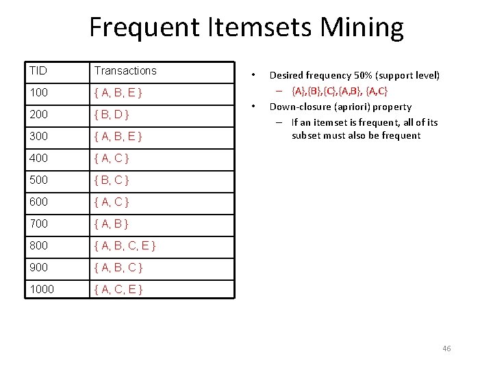
Frequent Itemsets Mining TID Transactions 100 { A, B, E } 200 { B, D } 300 { A, B, E } 400 { A, C } 500 { B, C } 600 { A, C } 700 { A, B } 800 { A, B, C, E } 900 { A, B, C } 1000 { A, C, E } • • Desired frequency 50% (support level) – {A}, {B}, {C}, {A, B}, {A, C} Down-closure (apriori) property – If an itemset is frequent, all of its subset must also be frequent 46

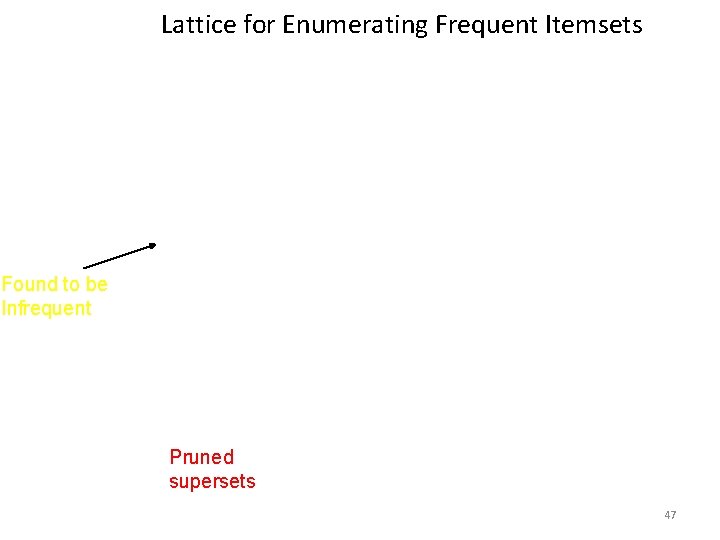
Lattice for Enumerating Frequent Itemsets Found to be Infrequent Pruned supersets 47

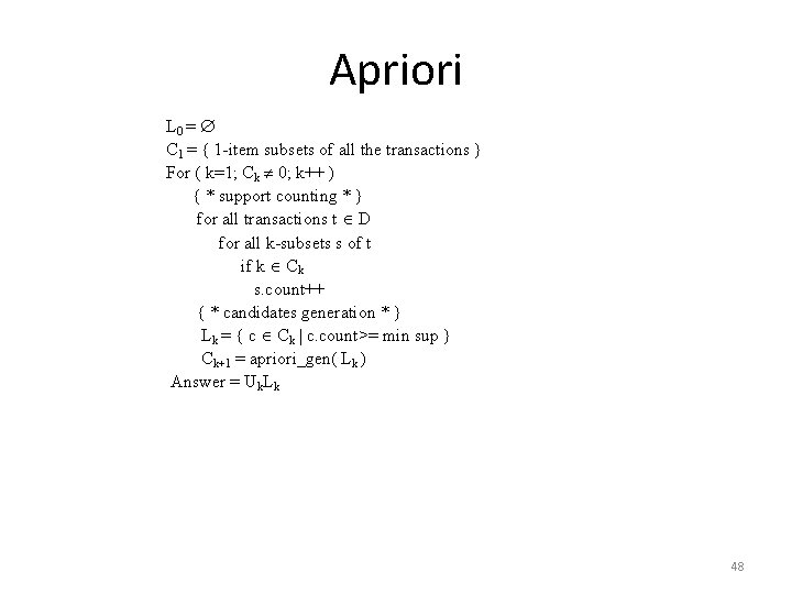
Apriori L 0 = C 1 = { 1 -item subsets of all the transactions } For ( k=1; Ck 0; k++ ) { * support counting * } for all transactions t D for all k-subsets s of t if k Ck s. count++ { * candidates generation * } Lk = { c Ck | c. count>= min sup } Ck+1 = apriori_gen( Lk ) Answer = Uk. Lk 48

Clustering • Clustering: Intuitively, finding clusters of points in the given data such that similar points lie in the same cluster • Can be formalized using distance metrics in several ways – Group points into k sets (for a given k) such that the average distance of points from the centroid of their assigned group is minimized • Centroid: point defined by taking average of coordinates in each dimension. – Another metric: minimize average distance between every pair of points in a cluster • Has been studied extensively in statistics, but on small data sets – Data mining systems aim at clustering techniques that can handle very large data sets – E. g. the Birch clustering algorithm! 49

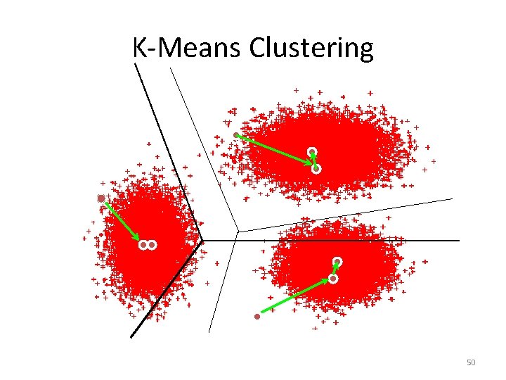
K-Means Clustering 50

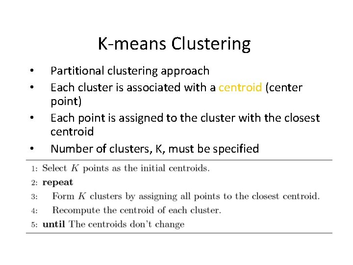
K-means Clustering • • • Partitional clustering approach Each cluster is associated with a centroid (center point) Each point is assigned to the cluster with the closest centroid Number of clusters, K, must be specified The basic algorithm is very simple

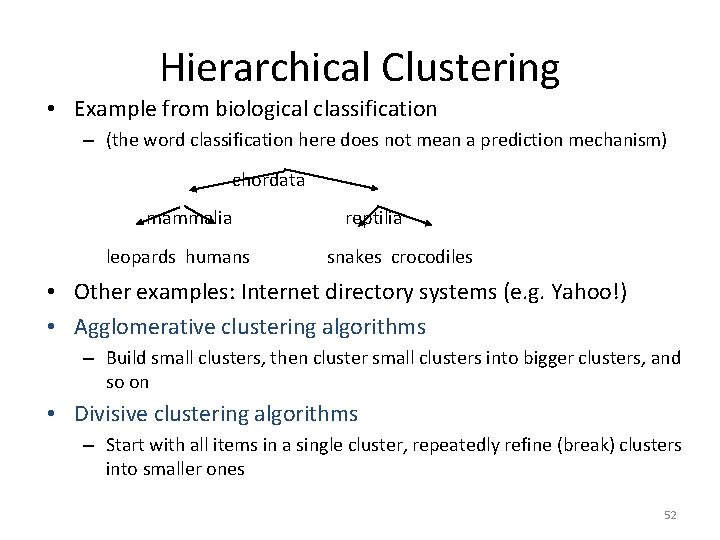
Hierarchical Clustering • Example from biological classification – (the word classification here does not mean a prediction mechanism) chordata mammalia leopards humans reptilia snakes crocodiles • Other examples: Internet directory systems (e. g. Yahoo!) • Agglomerative clustering algorithms – Build small clusters, then cluster small clusters into bigger clusters, and so on • Divisive clustering algorithms – Start with all items in a single cluster, repeatedly refine (break) clusters into smaller ones 52

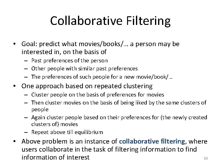
Collaborative Filtering • Goal: predict what movies/books/… a person may be interested in, on the basis of – Past preferences of the person – Other people with similar past preferences – The preferences of such people for a new movie/book/… • One approach based on repeated clustering – Cluster people on the basis of preferences for movies – Then cluster movies on the basis of being liked by the same clusters of people – Again cluster people based on their preferences for (the newly created clusters of) movies – Repeat above till equilibrium • Above problem is an instance of collaborative filtering, where users collaborate in the task of filtering information to find 53 information of interest

Other Types of Mining • Text mining: application of data mining to textual documents – cluster Web pages to find related pages – cluster pages a user has visited to organize their visit history – classify Web pages automatically into a Web directory • Data visualization systems help users examine large volumes of data and detect patterns visually – Can visually encode large amounts of information on a single screen – Humans are very good a detecting visual patterns 54

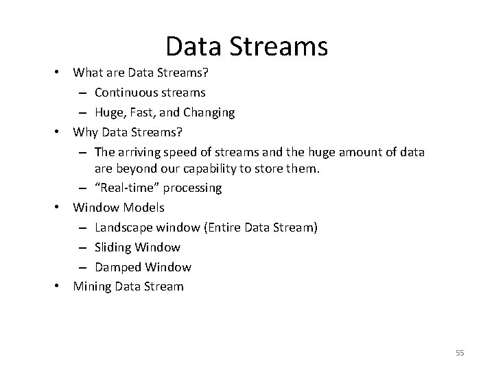
Data Streams • What are Data Streams? – Continuous streams – Huge, Fast, and Changing • Why Data Streams? – The arriving speed of streams and the huge amount of data are beyond our capability to store them. – “Real-time” processing • Window Models – Landscape window (Entire Data Stream) – Sliding Window – Damped Window • Mining Data Stream 55

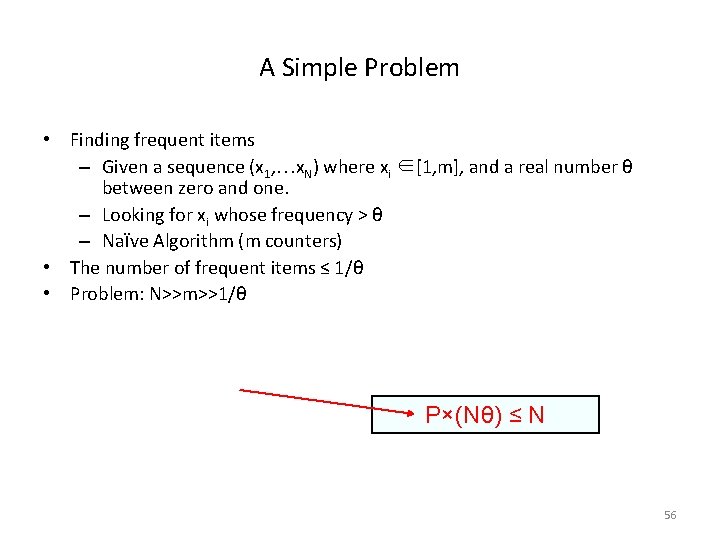
A Simple Problem • Finding frequent items – Given a sequence (x 1, …x. N) where xi ∈[1, m], and a real number θ between zero and one. – Looking for xi whose frequency > θ – Naïve Algorithm (m counters) • The number of frequent items ≤ 1/θ • Problem: N>>m>>1/θ P×(Nθ) ≤ N 56

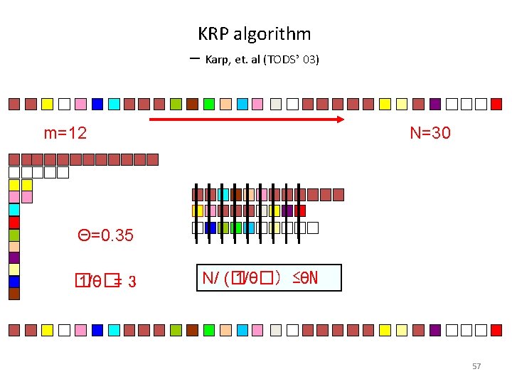
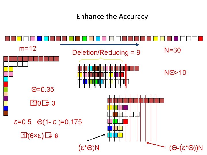
KRP algorithm ─ Karp, et. al (TODS’ 03) m=12 N=30 Θ=0. 35 � 1/θ�= 3 N/ (� 1/θ�) ≤θN 57

Enhance the Accuracy m=12 Deletion/Reducing = 9 N=30 NΘ>10 Θ=0. 35 � 1/θ�= 3 ε=0. 5 Θ(1 - ε )=0. 175 � 1/(θ×ε)�= 6 (ε*Θ)N 58 (Θ-(ε*Θ))N

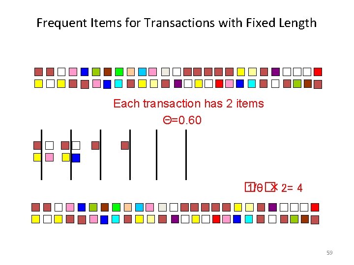
Frequent Items for Transactions with Fixed Length Each transaction has 2 items Θ=0. 60 � 1/θ� × 2= 4 59