Data Mining Data quality Missing values imputation using

Data Mining • Data quality • Missing values imputation using Mean, Median and k-Nearest Neighbor approach • Distance Measure

Data Quality • Data quality is a major concern in Data Mining and Knowledge Discovery tasks. • Why: At most all Data Mining algorithms induce knowledge strictly from data. • The quality of knowledge extracted highly depends on the quality of data. • There are two main problems in data quality: – Missing data: The data not present. – Noisy data: The data present but not correct. • Missing/Noisy data sources: – – Hardware failure. Data transmission error. Data entry problem. Refusal of responds to answer certain questions.

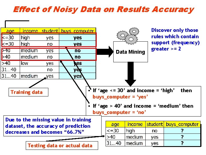
Effect of Noisy Data on Results Accuracy Data Mining Training data Discover only those rules which contain support (frequency) greater >= 2 • If ‘age <= 30’ and income = ‘high’ buys_computer = ‘yes’ then • If ‘age > 40’ and income = ‘medium’ then buys_computer = ‘no’ Due to the missing value in training dataset, the accuracy of prediction decreases and becomes “ 66. 7%” Testing data or actual data

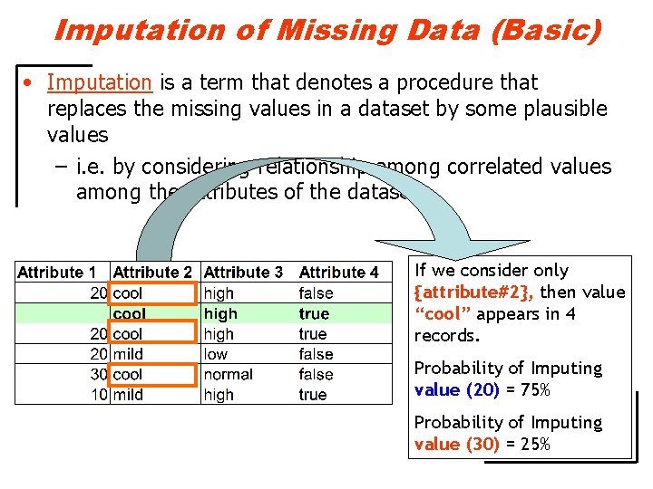
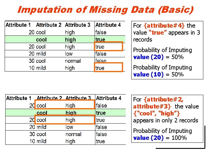
Imputation of Missing Data (Basic) • Imputation is a term that denotes a procedure that replaces the missing values in a dataset by some plausible values – i. e. by considering relationship among correlated values among the attributes of the dataset. If we consider only {attribute#2}, then value “cool” appears in 4 records. Probability of Imputing value (20) = 75% Probability of Imputing value (30) = 25%

Imputation of Missing Data (Basic) For {attribute#4} the value “true” appears in 3 records Probability of Imputing value (20) = 50% Probability of Imputing value (10) = 50% For {attribute#2, attribute#3} the value {“cool”, “high”} appears in only 2 records Probability of Imputing value (20) = 100%

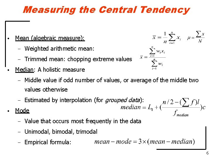
Measuring the Central Tendency • • Mean (algebraic measure): – Weighted arithmetic mean: – Trimmed mean: chopping extreme values Median: A holistic measure – Middle value if odd number of values, or average of the middle two values otherwise – • Estimated by interpolation (for grouped data): Mode – Value that occurs most frequently in the data – Unimodal, bimodal, trimodal – Empirical formula: 6

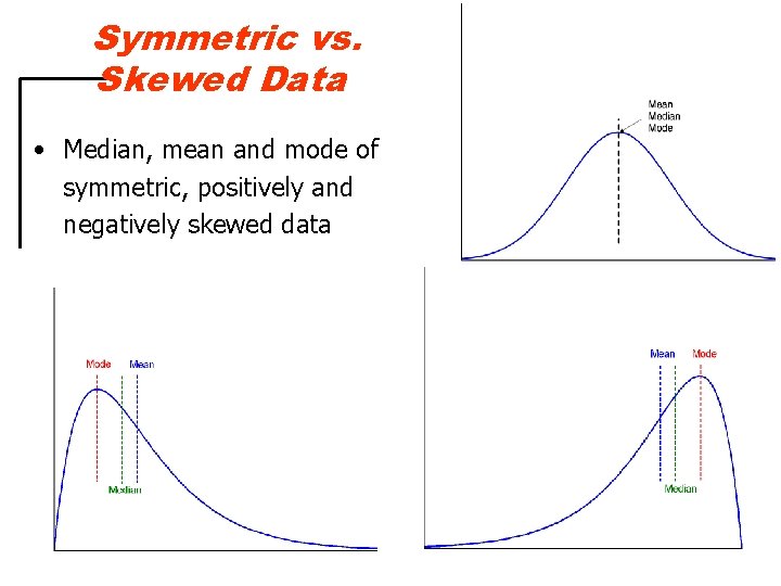
Symmetric vs. Skewed Data • Median, mean and mode of symmetric, positively and negatively skewed data 7

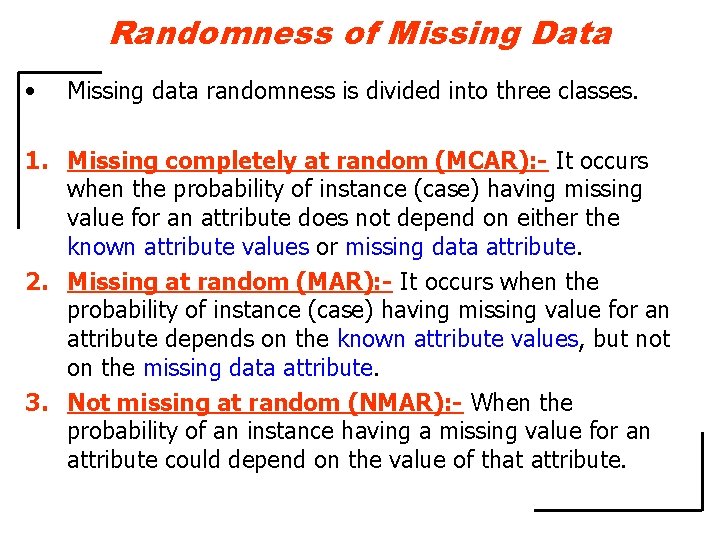
Randomness of Missing Data • Missing data randomness is divided into three classes. 1. Missing completely at random (MCAR): - It occurs when the probability of instance (case) having missing value for an attribute does not depend on either the known attribute values or missing data attribute. 2. Missing at random (MAR): - It occurs when the probability of instance (case) having missing value for an attribute depends on the known attribute values, but not on the missing data attribute. 3. Not missing at random (NMAR): - When the probability of an instance having a missing value for an attribute could depend on the value of that attribute.

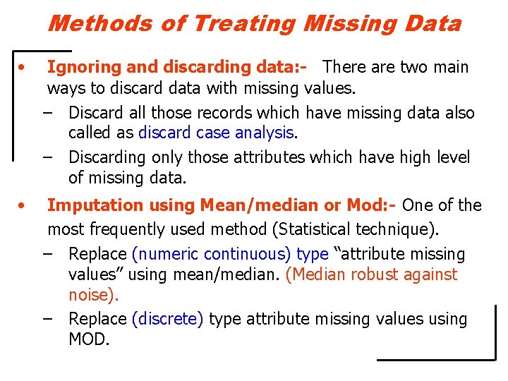
Methods of Treating Missing Data • Ignoring and discarding data: - There are two main ways to discard data with missing values. – Discard all those records which have missing data also called as discard case analysis. – Discarding only those attributes which have high level of missing data. • Imputation using Mean/median or Mod: - One of the most frequently used method (Statistical technique). – Replace (numeric continuous) type “attribute missing values” using mean/median. (Median robust against noise). – Replace (discrete) type attribute missing values using MOD.

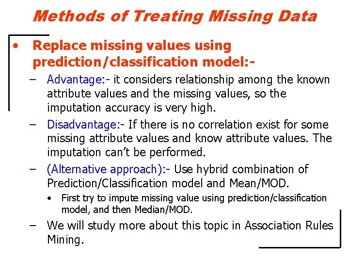
Methods of Treating Missing Data • Replace missing values using prediction/classification model: – Advantage: - it considers relationship among the known attribute values and the missing values, so the imputation accuracy is very high. – Disadvantage: - If there is no correlation exist for some missing attribute values and know attribute values. The imputation can’t be performed. – (Alternative approach): - Use hybrid combination of Prediction/Classification model and Mean/MOD. • First try to impute missing value using prediction/classification model, and then Median/MOD. – We will study more about this topic in Association Rules Mining.

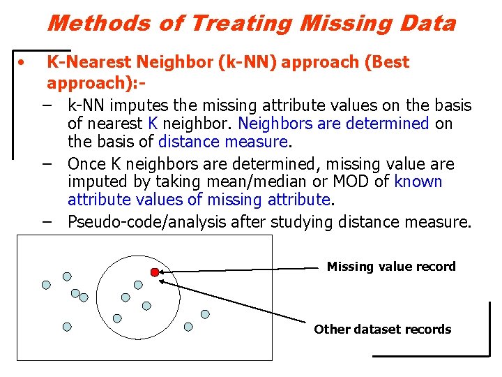
Methods of Treating Missing Data • K-Nearest Neighbor (k-NN) approach (Best approach): – k-NN imputes the missing attribute values on the basis of nearest K neighbor. Neighbors are determined on the basis of distance measure. – Once K neighbors are determined, missing value are imputed by taking mean/median or MOD of known attribute values of missing attribute. – Pseudo-code/analysis after studying distance measure. Missing value record Other dataset records

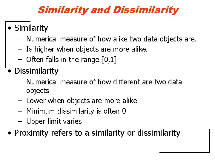
Similarity and Dissimilarity • Similarity – Numerical measure of how alike two data objects are. – Is higher when objects are more alike. – Often falls in the range [0, 1] • Dissimilarity – Numerical measure of how different are two data objects – Lower when objects are more alike – Minimum dissimilarity is often 0 – Upper limit varies • Proximity refers to a similarity or dissimilarity

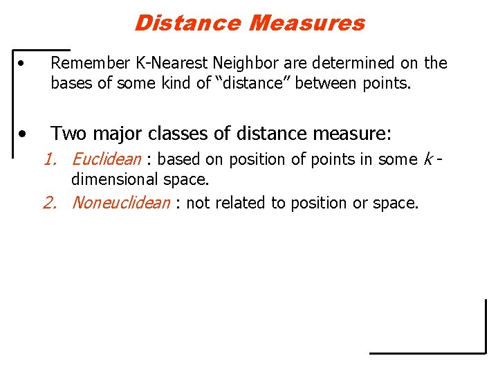
Distance Measures • Remember K-Nearest Neighbor are determined on the bases of some kind of “distance” between points. • Two major classes of distance measure: 1. Euclidean : based on position of points in some k dimensional space. 2. Noneuclidean : not related to position or space.

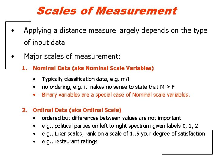
Scales of Measurement • Applying a distance measure largely depends on the type of input data • Major scales of measurement: 1. Nominal Data (aka Nominal Scale Variables) • • • Typically classification data, e. g. m/f no ordering, e. g. it makes no sense to state that M > F Binary variables are a special case of Nominal scale variables. 2. Ordinal Data (aka Ordinal Scale) • ordered but differences between values are not important • e. g. , political parties on left to right spectrum given labels 0, 1, 2 • e. g. , Liker scales, rank on a scale of 1. . 5 your degree of satisfaction • e. g. , restaurant ratings

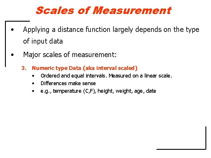
Scales of Measurement • Applying a distance function largely depends on the type of input data • Major scales of measurement: 3. Numeric type Data (aka interval scaled) • Ordered and equal intervals. Measured on a linear scale. • Differences make sense • e. g. , temperature (C, F), height, weight, age, date

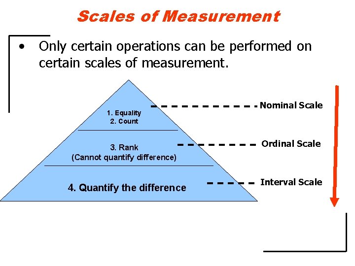
Scales of Measurement • Only certain operations can be performed on certain scales of measurement. 1. Equality 2. Count 3. Rank (Cannot quantify difference) 4. Quantify the difference Nominal Scale Ordinal Scale Interval Scale

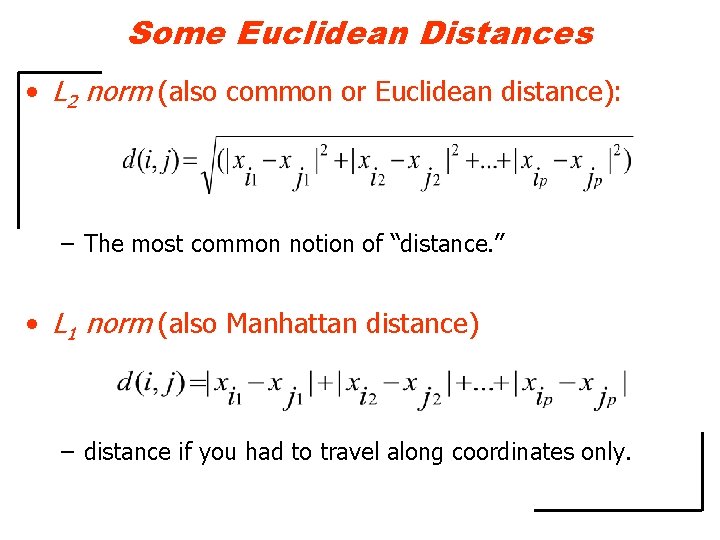
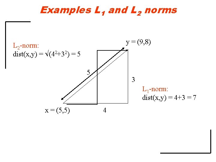
Some Euclidean Distances • L 2 norm (also common or Euclidean distance): – The most common notion of “distance. ” • L 1 norm (also Manhattan distance) – distance if you had to travel along coordinates only.

Examples L 1 and L 2 norms y = (9, 8) L 2 -norm: dist(x, y) = (42+32) = 5 5 3 L 1 -norm: dist(x, y) = 4+3 = 7 x = (5, 5) 4

Another Euclidean Distance • L∞ norm : d(x, y) = the maximum of the differences between x and y in any dimension.

Non-Euclidean Distances • Jaccard measure for binary vectors • Cosine measure = angle between vectors from the origin to the points in question. • Edit distance = number of inserts and deletes to change one string into another.

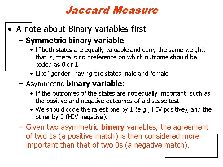
Jaccard Measure • A note about Binary variables first – Symmetric binary variable • If both states are equally valuable and carry the same weight, that is, there is no preference on which outcome should be coded as 0 or 1. • Like “gender” having the states male and female – Asymmetric binary variable: • If the outcomes of the states are not equally important, such as the positive and negative outcomes of a disease test. • We should code the rarest one by 1 (e. g. , HIV positive), and the other by 0 (HIV negative). – Given two asymmetric binary variables, the agreement of two 1 s (a positive match) is then considered more important than that of two 0 s (a negative match).

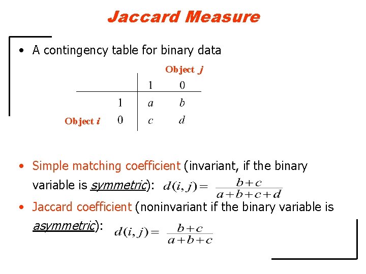
Jaccard Measure • A contingency table for binary data Object j Object i • Simple matching coefficient (invariant, if the binary variable is symmetric): • Jaccard coefficient (noninvariant if the binary variable is asymmetric):

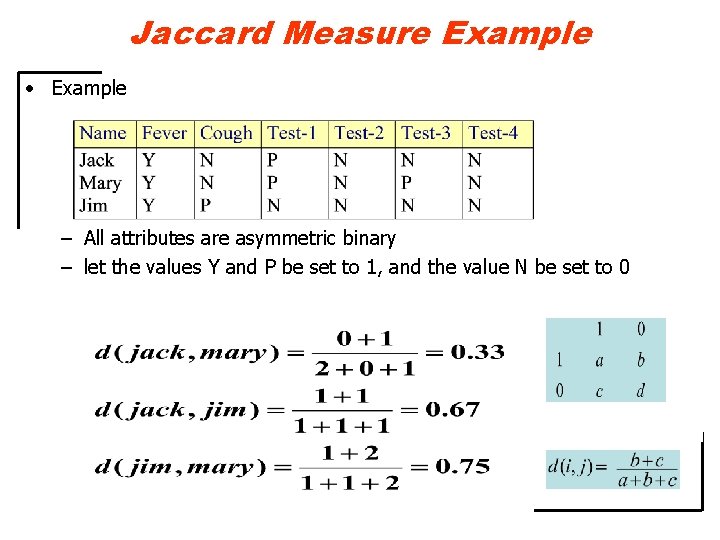
Jaccard Measure Example • Example – All attributes are asymmetric binary – let the values Y and P be set to 1, and the value N be set to 0

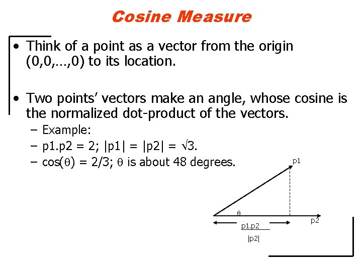
Cosine Measure • Think of a point as a vector from the origin (0, 0, …, 0) to its location. • Two points’ vectors make an angle, whose cosine is the normalized dot-product of the vectors. – Example: – p 1. p 2 = 2; |p 1| = |p 2| = 3. – cos( ) = 2/3; is about 48 degrees. p 1 dist(p 1, p 2) = = arccos(p 1. p 2/|p 2||p 1|) p 1. p 2 |p 2| p 2

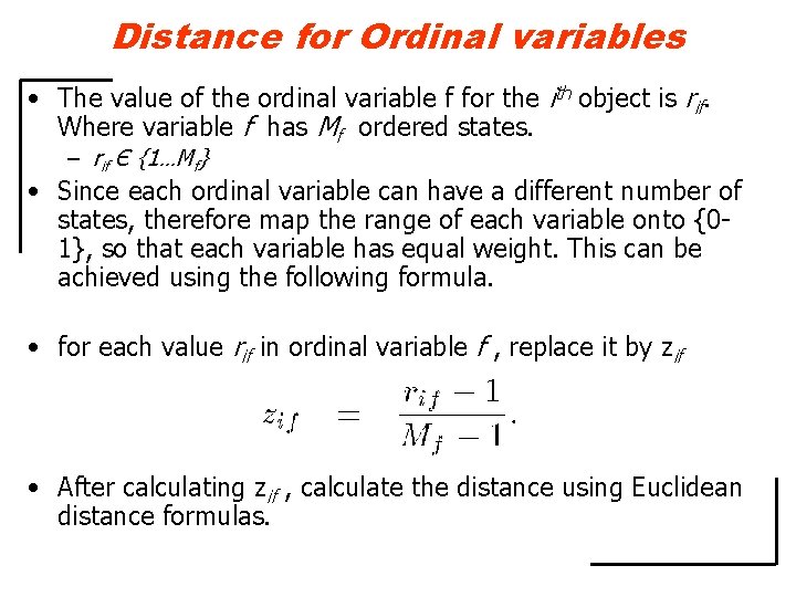
Distance for Ordinal variables • The value of the ordinal variable f for the ith object is rif. Where variable f has Mf ordered states. – rif Є {1…Mf} • Since each ordinal variable can have a different number of states, therefore map the range of each variable onto {01}, so that each variable has equal weight. This can be achieved using the following formula. • for each value rif in ordinal variable f , replace it by zif • After calculating zif , calculate the distance using Euclidean distance formulas.

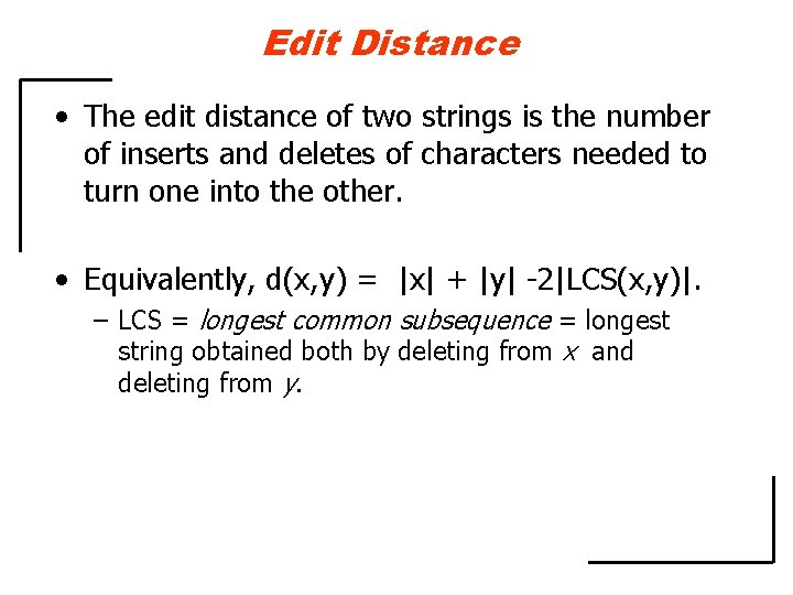
Edit Distance • The edit distance of two strings is the number of inserts and deletes of characters needed to turn one into the other. • Equivalently, d(x, y) = |x| + |y| -2|LCS(x, y)|. – LCS = longest common subsequence = longest string obtained both by deleting from x and deleting from y.

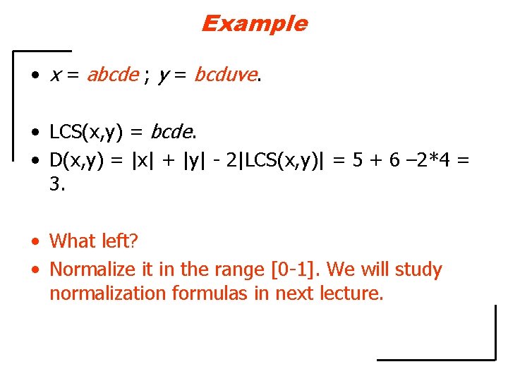
Example • x = abcde ; y = bcduve. • LCS(x, y) = bcde. • D(x, y) = |x| + |y| - 2|LCS(x, y)| = 5 + 6 – 2*4 = 3. • What left? • Normalize it in the range [0 -1]. We will study normalization formulas in next lecture.

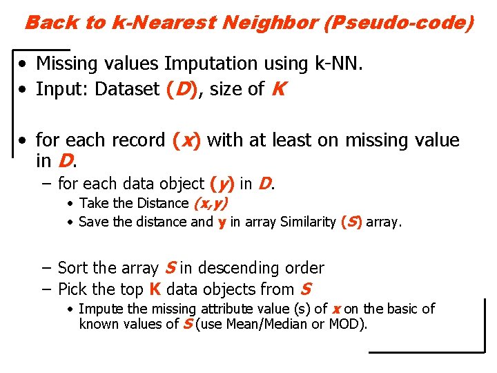
Back to k-Nearest Neighbor (Pseudo-code) • Missing values Imputation using k-NN. • Input: Dataset (D), size of K • for each record (x) with at least on missing value in D. – for each data object (y) in D. • Take the Distance (x, y) • Save the distance and y in array Similarity (S) array. – Sort the array S in descending order – Pick the top K data objects from S • Impute the missing attribute value (s) of x on the basic of known values of S (use Mean/Median or MOD).

K-Nearest Neighbor Drawbacks • The major drawbacks of this approach are the – Choice of selecting exact distance functions. – Considering all attributes when attempting to retrieve the similar type of examples. – Searching through all the dataset for finding the same type of instances. – Algorithm Cost: ?

Noisy Data • Noise: Random error, Data Present but not correct. – Data Transmission error – Data Entry problem • Removing noise – Data Smoothing (rounding, averaging within a window). – Clustering/merging and Detecting outliers. • Data Smoothing – First sort the data and partition it into (equi-depth) bins. – Then the values in each bin using Smooth by Bin Means, Smooth by Bin Median, Smooth by Bin Boundaries, etc.

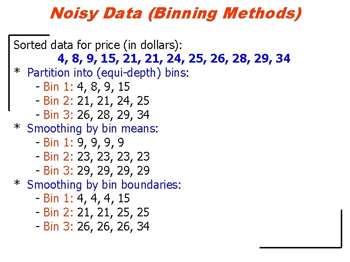
Noisy Data (Binning Methods) Sorted data for price (in dollars): 4, 8, 9, 15, 21, 24, 25, 26, 28, 29, 34 * Partition into (equi-depth) bins: - Bin 1: 4, 8, 9, 15 - Bin 2: 21, 24, 25 - Bin 3: 26, 28, 29, 34 * Smoothing by bin means: - Bin 1: 9, 9, 9, 9 - Bin 2: 23, 23, 23 - Bin 3: 29, 29, 29 * Smoothing by bin boundaries: - Bin 1: 4, 4, 4, 15 - Bin 2: 21, 25, 25 - Bin 3: 26, 26, 34

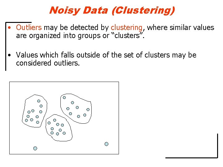
Noisy Data (Clustering) • Outliers may be detected by clustering, where similar values are organized into groups or “clusters”. • Values which falls outside of the set of clusters may be considered outliers.

References – G. Batista and M. Monard, “The study of K-Nearest Neighbor as a Imputation Method”, 2002. (I will placed at the course folder) – “CS 345 --- Lecture Notes”, by Jeff D Ullman at Stanford. http: //www-db. stanford. edu/~ullman/cs 345 -notes. html – Vipin Kumar’s course in data mining offered at University of Minnesota – official text book slides of Jiawei Han and Micheline Kamber, “Data Mining: Concepts and Techniques”, Morgan Kaufmann Publishers, August 2000.