DATA WAREHOUSE DATA MINING AND DATA WARE HOUSING

DATA WAREHOUSE

DATA MINING AND DATA WARE HOUSING UNIT - I Introduction – Data warehouse delivery method – System Process – Typical process flow within a data warehouse – query management process – process architecture – meta data – data marting. UNIT - II Design aspects – Designing dimension tables – Designing starflake schema – Multi Dimensional Schema – Partition Strategy, Aggregator – Data marting – Meta Data – System Data Warehouse, Process – Load Manager UNIT - III Hardware and operational design – server hardware – network hardware – parallel technology – security input and design of hardware – backup and recovery – service level agreement – operating the hardware

DIMENSIONAL MODELLING It is the design concept used by many Data Warehouse designers to build their Data Warehouse. It contains two types of tables 1. FACT TABLE 2. DIMENSION TABLE FACT TABLE Fact Tables contains the measurements, or metrics or facts of the business process. If your business process is SALES, then the measurement of this business process such as “monthly sales number” is captured into the fact table. In addition to measurements, the only other things a fact table contains are foreign keys for the dimension table

DIMENSION TABLE Context of measurements are represented in dimension tables. Context of measurement such as who, what, were, when, how of measurement (subject) If your business process is sales (monthly sales no) then measurement can be location (where), time (when), product sold (what) DIMENSION ATTRIBUTE This are various columns in a dimension table. In a location dimension, the attributes can be location code, state, country, zip code. Before designing your DWH, you need to decide what this DWH contains. Ex if you want to build a DWH containing Sales, across multiple locations, across time and across products then your dimensions would 1) Location 2) Time 3) Product

Each dimension table contains data for one dimension “ A SCHEMA IS A FACT TABLE PLUS ITS RELATED DIMENSION TABLES”. Visually, a dimension schema looks very much like a star, hence the term STAR SCHEMA used to describe dimensional model. Fact table reside at the center of the schema, and their dimensions are typically drawn around it.

TIME PRODUCT FACT TABLE (SALES) CLIENT LOCATION

STAR SCHEMA : A normalized multi-dimensional model in which each disjoint dimension is represented by a single table. One key principles of dimensional modeling is the use of fully normalized fact tables together with fully de-normalized dimensional tables. Each dimension table contains data for one dimension. Why dimensions should be de-normalized ?

In order to query for all locations that are in country ‘USA’. In OLTP you store location data in multiple tables. For Ex : 3 Tables LOCATION TABLE STATES TABLE COUNTRIES TABLE FIELD TYPE Loc_id int (4) State_id int (4) Country_id int (4) Loc_code varchar(5) State_name varchar(50) Country_name varchar(50) Loc_name varchar(30) State_id int (4) Country_id int (4)

Now in OLTP the location data may be be spanned across multiple tables. SQL will look like. SELECT * FROM Location, States, Countries where locations. state_id = states. state_id AND Locations. country_id = country_id AND Country_name = ‘USA’ RELATION IN OLTP Locations PK Countries PK country_id country_nam e Location_id Loc_name FK 2 State_id FK 1 County_id States PK State_id

But in OLAP you need to De-Normalized all the data into a single table Dim_id Loc_cod Name e State_name Country_nam 1001 IL 01 Chicago Loop Illinois USA 1002 ILo 2 Brooklyn Illinois USA 1003 NY 01 Toronto Ontario CANADA 1004 TO 01 Mexico City Distrito MEXICO e Data repeated but makes querying optimized and reduces the query time.

Properties of Fact and Dimension Tables : Property Location Table Product Table Time Table Sales Table TABLE TYPE Dimension DIM FACT One Record is Location One Product One Day SALES Per LOCATION Per PRODUCT Per DAY Key Product Key Time Key Client Key + Product Key + Time Key Location Key

Advantages of the STAR Schema: n n Easy for Users to Understand Optimizes Navigation Most Suitable for Query Processing STARjoin and STARindex

Easy for Users to Understand n n n Users of decision support systems such as data warehouses are different. Here users themselves will formulate queries. When they interact with the data warehouse through third-party query tools, the users should know what to ask for. They must gain a familiarity with what data is available to them in the data warehouse. They must have an understanding of the data structures and how the various pieces are associated with one another in the overall scheme. The STAR schema reflects exactly how the users think and need data for querying and analysis. When you explain to the users that the units of product A are stored in the fact table and point out the relationship of this piece of data to each dimension table, the user readily understand the connections. That is because the STAR schema defines the join paths in exactly the same way users normally visualize the relationships.

Optimizes Navigation n In a database schema, what is the purpose of the relationships or connections among the data entities? A major advantage of the STAR schema is that it optimizes the navigation through the database. Example: Assume you are the service manager at an automobile dealership selling GM automobiles. You noticed a high incidence of chipped white paint on the Corvettes in January 2000. You need a tool to analyze such defects, determine the underlying causes, and resolve the problems.

TIME (Model year) COMPONENT (Part info) PRODUCT (The make, model, and trim package) DEFECTS (No. Of defects) SUPPLIER (Supplier parts) PROBLEM (Types of problems) Figure: The STAR schema optimizes navigation v. Now it is easy to determine the supplier causing the chipped paint on the pearl white corvettes. v. Four arrows pointing to the fact table from the four dimension tables show you will navigate to the rows in the fact table by isolating the Corvette from the product dimension

Most Suitable for Query Processing n Let us form a simple query on the STAR schema for the order analysis. What is the total extended cost of product A sold to customers in San Francisco during January 2000? v San Francisco. Then, from the fact table, select only those rows that are related to these customer dimension rows. This is first set of rows from the fact tables. the me mension in rows month Next, table where select the v is January 2000. Select from the first result set of fact table rows. v product dimension table where the product is product A v the selected product dimension rows.

STARjoin and STARindex n The STAR schema allows the query processor software to use better execution plans. n STARjoin can join more than two tables in a single operation. n STARindex is a specialized index to accelerate joins performance. These are indexes created on one or more foreign keys of the fact table.

SNOW FLAKE SCHEMA : A normalized multidimensional model in which each disjoint dimension is represented by one or more hierarchical tables FACT SNOWFLAKE STAR DIMENSIONS

FACT SNOWFLAKE STAR DIMENSIONS LOCATIONS DEPARTM SALES TRANSACTIONS LOCATIONS PRODUCTS REGION BUSINESS UNIT STYLE COLOR TIME PRODUCT SIZE WEEK MONTH SUMMER SALES EASTER SALES

Advantages n Small saving in storage space n Normalized structure are easier to update and maintain. Disadvantages n n n Schema less intuitive and end-users are put off by the complexity. Ability to browse through the contents difficult. Degraded query performance because of additional joins.

Fact constellation: Sophisticated applications may require multiple fact tables to share dimension tables. This kind of schema can be viewed as a collection of stars, and hence is called a galaxy schema or a fact constellation. Multiple fact tables that share many dimension tables Booking and Checkout may share many dimension tables in the hotel industry

Examples for Defining Star, Snowflake, and Fact Constellation Schemas Data warehouses and data marts can be defined using two language primitives, one for cube definition and one for dimension definition. $The cube definition statement has the following syntax: define cube <cube name> [<dimension list>]: <measure list> $The dimension definition statement has the following syntax: define dimension <dimension name> as (<attribute dimension list>) or > Star schema definition. DMQL for the above diagram: define cube sales star [time, item, branch, location]: dollars sold = sum(sales in dollars), units sold = count(*) define dimension time as (time key, day of week, month, quarter, year)

define dimension item as (item key, item name, brand, type, supplier type) define dimension branch as (branch key, branch name, branch type) define dimension location as (location key, street, city, province or state, country) > Snowflake schema definition. DMQL for the above diagram define cube sales snowflake [time, item, branch, location]: dollars sold = sum(sales in dollars), units sold = count(*) define dimension time as (time key, day of week, month, quarter, year) define dimension item as (item key, item name, brand, type, supplier (supplier key, supplier type)) define dimension branch as (branch key, branch name, branch type) define dimension location as (location key, street, city (city key, city, province or state, country))

> Fact constellation schema def. DMQL for the above diagram define cube sales [time, item, branch, location]: dollars sold = sum(sales in dollars), units sold = count(*) define dimension time as (time key, day of week, month, quarter, year) define dimension item as (item key, item name, brand, type, supplier type) define dimension branch as (branch key, branch name, branch type) define dimension location as (location key, street, city, province or state, country) define cube shipping [time, item, shipper, from location, to location]: dollars cost = sum(cost in dollars), units shipped = count(*) define dimension time as time in cube sales define dimension item as item in cube sales define dimension shipper as (shipper key, shipper name, location as location in cube sales, shipper type) define dimension from location as location in cube sales define dimension to location as location in cube sales

Measures: Their Categorization and Computation Distributive if the result derived by applying the function to n aggregate values is the same as that derived by applying the function on all the data without partitioning. E. g. , count(), sum(), min(), max() Algebraic if it can be computed by an algebraic function with M arguments (where M is a bounded integer), each of which is obtained by applying a distributive aggregate function. E. g. , avg(), min_N(), standard_deviation() Holistic if there is no constant bound on the storage size needed to describe a sub aggregate. E. g. , median(), mode(), rank()

Concept Hierarchies • A concept hierarchy defines a sequence of mappings from a set of low-level concepts to higher-level, more general concepts. • Many concept hierarchies are implicit within the database schema. • A concept hierarchy that is a total or partial order among attributes in a database schema is called a schema hierarchy. Specification of hierarchies Schema hierarchy day < {month < quarter; week} < year Set_grouping hierarchy {1. . 10} < inexpensive

• Concept hierarchies that are common to many applications may be predefined in the data mining system, such as the concept hierarchy for time. • Data mining systems should provide users with the flexibility to tailor predefined hierarchies according to their particular needs. • Concept hierarchies may also be defined by discretizing or grouping values for a given dimension or attribute, resulting in a setgrouping hierarchy. • There may be more than one concept hierarchy for a given attribute or dimension, based on different user viewpoints. • Concept hierarchies may be provided manually by system users, domain experts, or knowledge engineers, or may be automatically generated based on statistical analysis of the data distribution. • Concept hierarchies allow data to be handled at varying levels of abstraction.

Figure : A concept hierarchy for the dimension location.

Figure : Hierarchical and lattice structures of attributes in warehouse dimensions: (a) a hierarchy for location; (b) a lattice for time.

A Multidimensional Data Model Data warehouses and OLAP tools are based on a multidimensional data model. This model views data in the form of a data cube. From Tables and Spreadsheets to Data Cubes “What is a data cube? ” A data cube allows data to be modeled and viewed in multiple dimensions. It is defined by dimensions and facts. A 2 -D view of sales data for XYZ according to the dimensions time and item, where the sales are from branches located in the city of Hyderabad. Location= “Hyderabad” Item (type) Time (Quarter) Home Theater Computer Mobile Phones Television Q 1 45 101 67 23 Q 2 43 34 86 54 Q 3 23 156 129 12 Q 4 12 12 156 28

A 3 -D view of sales data for XYZ according to the dimensions time, item and location. Location= “Hyderabad” Location= “Chennai” Location= “Mumbai” Item (type) Time HT Comp Mobile TV Q 1 45 101 67 23 25 76 34 36 43 34 87 45 Q 2 43 34 86 54 40 45 67 48 112 45 119 67 Q 3 23 156 129 12 32 56 189 15 67 58 45 32 Q 4 12 12 156 28 14 27 16 27 46 67 134 23 A 3 -D data cube representation of the data in above Table, according to the dimensions time, item, and location.

Pr od TV PC VCR sum 1 Qtr 2 Qtr Date 3 Qtr 4 Qtr sum Total annual sales of TV in U. S. A Canada Mexico sum Country uc t A Sample Data Cube

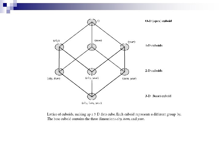
Cuboids Corresponding to the Cube all 0 -D(apex) cuboid product, date country product, country 1 -D cuboids date, country 2 -D cuboids product, date, country 3 -D(base) cuboid

Browsing a Data Cube n n n Visualization OLAP capabilities Interactive manipulation

Multidimensional Schemas Class of decision support queries, that analyze data by representing facts and dimensions within a multidimensional cube. Effects as each dimension will occupy an axis and values within cubes corresponds to factual transformations. It is used to view the cubes, pivot point, slice and dice. Ex : Retail Sales Analysis using a cubical representation of products by store by day in a 3 -D cube with 3 axes representing Product, Store & Day Time Location Product

Some operations in the multidimensional data model n n n Roll-up(drill-up)-Performs aggregation on a data cube, either by climbing up a concept hierarchy for a dimension or by dimension reduction. Drill-down- Reverse of roll-up operation. It navigates from less details data to more detailed data. Slice- Performs a selection on one dimension of the given cube, resulting in a sub-cube. Dice- Define a sub-cube by performing a selection on two or more dimensions. Pivot(rotate)- is a visualization operation that rotates the data axes in a view , in order to provide an alternative presentation of data.

Toronto Vancover Q 1 Dice for (location=”Toronto “ or “vancover”) and (time=”Q 1” or “Q 2”) and (item=”H. E” or “comp) Chicago Location 440 NY 156 Toronto (Cities) Vancover 395 Q 1 Time (quarters) 605 825 14 400 Q 2 H. E. comp Items (types) H. E C omp Phon e Q 2 Security Q 3 605 825 14 400 Chicago NY Toronto Vancover Q 4 Pivot Home comp phone security entertainment Items (types) slice for time “Q 1” Chicago NY Toronto Vancover 605 825 14 400 Home comp phone security entertainment

Location (Cities) Chicago 440 NY 156 Toronto 395 Vancover Q 1 605 825 14 400 Q 2 Time (quarters) time(from quarters to months) Chicago NY Toronto Vancover Q 3 Q 4 Roll-up On location (from cities to country) Drill-down on Home comp phone security entertainment Items (types) June July August USA Canada Time (months) Q 1 Q 2 Q 3 Q 4 H. E comp phone security Items (types) Jan Feb Mar App May Sep Oct Nov Dec H. E comp phone security Items (types)

Product by store by day cube The point of intersection of all axes represents the actual number of sales for a specific product, in a specific store, on a specific day. Also alternatively if we wish to view sum of all sales by a specific store and a specific day. Aggregation function would be applied by slice and dice Sum of all (Products) Location Sum (Products)

Data. Warehouse Architecture Steps for the Design and Construction of Data. Warehouses : A) Business Analysis Framework Four different views regarding the design of a data warehouse must be considered: the top-down view, the data source view, the data warehouse view, and the business query view. The top-down view allows the selection of the relevant information necessary for the data warehouse. This information matches the current and future business needs. The data source view exposes the information being captured, stored, and managed by operational systems. This information may be documented at various levels of detail and accuracy, from individual data source tables to integrated data source tables. Data sources are often modeled by traditional data modeling techniques, such as the entity-relationship model or CASE (computer-aided software engineering) tools.

The data warehouse view includes fact tables and dimension tables. It represents the information that is stored inside the data warehouse, including precalculated totals and counts, as well as information regarding the source, date, and time of origin, added to provide historical context. Finally, the business query view is the perspective of data in the data warehouse from the viewpoint of the end user.

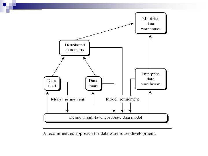
B) The Process of Data Warehouse Design In general, the warehouse design process consists of the following steps: 1. Choose a business process to model, for example, orders, invoices, shipments, inventory, account administration, sales, or the general ledger. If the business process is organizational and involves multiple complex object collections, a data warehouse model should be followed. However, if the process is departmental and focuses on the analysis of one kind of business process, a data mart model should be chosen. 2. Choose the grain of the business process. The grain is the fundamental, atomic level of data to be represented in the fact table for this process, for example, individual transactions, individual daily snapshots, and so on.

3. Choose the dimensions that will apply to each fact table record. Typical dimensions are time, item, customer, supplier, warehouse, transaction type, and status. 4. Choose the measures that will populate each fact table record. Typical measures are numeric additive quantities like dollars sold and units sold.

2. A Three-Tier Data Warehouse Architecture

1. The bottom tier is a warehouse database server that is almost always a relational database system. Back-end tools and utilities are used to feed data into the bottom tier from operational databases or other external sources 2. The middle tier is an OLAP server that is typically implemented using either (1) a relational OLAP (ROLAP) model, that is, an extended relational DBMS that maps operations on multidimensional data to standard relational operations; or (2) a multidimensional OLAP (MOLAP) model, that is, a special-purpose server that directly implements multidimensional data and operations. 3. The top tier is a front-end client layer, which contains query and reporting tools, analysis tools, and/or data mining tools (e. g. , trend analysis, prediction, and so on).

Enterprise warehouse: An enterprise warehouse collects all of the information about subjects spanning the entire organization. Data mart: A data mart contains a subset of corporate-wide data that is of value to a specific group of users. Virtual warehouse: A virtual warehouse is a set of views over operational databases.

3. Data. Warehouse Back-End Tools and Utilities Data warehouse systems use back-end tools and utilities to populate and refresh their data. These tools and utilities include the following functions: Data extraction, which typically gathers data frommultiple, heterogeneous, and external sources Data cleaning, which detects errors in the data and rectifies them when possible Data transformation, which converts data from legacy or host format to warehouse format. Load, which sorts, summarizes, consolidates, computes views, checks integrity, builds indices and partitions Refresh, which propagates the updates from the data sources to the warehouse

Metadata Repository Metadata are data about data. When used in a data warehouse, metadata are the data that define warehouse objects. Additional metadata are created and captured for timestamping any extracted data, the source of the extracted data, and missing fields that have been added by data cleaning or integration processes. A metadata repository should contain the following: 1) A description of the structure of the data warehouse, which includes the warehouse schema, view, dimensions, hierarchies, and derived data definitions, as well as data mart locations and contents 2) Operational metadata, which include data lineage (history of migrated data and the sequence of transformations applied to it), currency of data (active, archived, or purged), and monitoring information (warehouse usage statistics, error reports, and audit trails)

3) The algorithms used for summarization, which include measure and dimension definition algorithms, data on granularity, partitions, subject areas, aggregation, summarization, and predefined queries and reports 4) The mapping from the operational environment to the data warehouse, which includes source databases and their contents, gateway descriptions, data partitions, data extraction, cleaning, transformation rules and defaults, data refresh and purging rules, and security (user authorization and access control) 5) Data related to system performance, which include indices and profiles that improve data access and retrieval performance, in addition to rules for the timing and scheduling of refresh, update, and replication cycles 6) Business metadata, which include business terms and definitions, data ownership information, and charging policies

A data warehouse contains different levels of summarization, of which metadata is one type. Other types include current detailed data (which are almost always on disk), older detailed data (which are usually on tertiary storage), lightly summarized data and highly summarized data (which may or may not be physically housed). Metadata play a very different role than other data warehouse data and are important for many reasons. Metadata should be stored and managed persistently (i. e. , on disk).

Types of OLAP Servers: ROLAP versus MOLAP versus HOLAP Relational OLAP (ROLAP) servers: These are the intermediate servers that stand in between a relational back-end server and client front-end tools. They use a relational or extended-relational. DBMS to store and manage warehouse data, and OLAP middleware to support missing pieces. ROLAP servers include optimization for each DBMS back end, implementation of aggregation navigation logic, and additional tools and services. ROLAP technology tends to have greater scalability than MOLAP technology. The DSS server of Microstrategy, for example, adopts the ROLAP approach.

Multidimensional OLAP (MOLAP) servers: These servers support multidimensional views of data through arraybased multidimensional storage engines. They map multidimensional views directly to data cube array structures. The advantage of using a data cube is that it allows fast indexing to precomputed summarized data. Notice that with multidimensional data stores, the storage utilizationmay be lowif the data set is sparse. In such cases, sparse matrix compression techniques should be explored. Many MOLAP servers adopt a two-level storage representation to handle dense and sparse data sets: denser subcubes are identified and stored as array structures, whereas sparse subcubes employ compression technology for efficient storage utilization.

Hybrid OLAP (HOLAP) servers: The hybrid OLAP approach combines ROLAP and MOLAP technology, benefiting from the greater scalability of ROLAP and the faster computation of MOLAP. For example, a HOLAP server may allow large volumes of detail data to be stored in a relational database, while aggregations are kept in a separate MOLAP store. The Microsoft SQL Server 2000 supports a hybrid OLAP server. Specialized SQL servers: To meet the growing demand of OLAP processing in relational databases, some database system vendors implement specialized SQL servers that provide advanced query language and query processing support for SQL queries over star and snowflake schemas in a read-only environment.

Data. Warehouse Implementation Data warehouses contain huge volumes of data. OLAP servers demand that decision support queries be answered in the order of seconds. Therefore, it is crucial for data warehouse systems to support highly efficient cube computation techniques, access methods, and query processing techniques. Efficient Computation of Data Cubes At the core ofmultidimensional data analysis is the efficient computation of aggregations across many sets of dimensions. In SQL terms, these aggregations are referred to as group-by’s. Each group-by can be represented by a cuboid, where the set of group-by’s forms a lattice of cuboids defining a data cube.

a) The compute cube Operator and the Curse of Dimensionality One approach to cube computation extends SQL so as to include a compute cube operator. The compute cube operator computes aggregates over all subsets of the dimensions specified in the operation. This can require excessive storage space, especially for large numbers of dimensions. e. g: “Compute the sum of sales, grouping by city and item. ” syntax of DMQL: define cube sales cube [city, item, year]: sum(sales in dollars) For a cube with n dimensions, there a total of 2 n cuboids, including the base cuboid. A statement such as compute cube sales cube would explicitly instruct the system to compute the sales aggregate cuboids for all of the eight subsets of the set fcity, item, yearg, including the empty subset. A cube computation operator was first proposed and studied by Gray et al.

“How many cuboids are there in an n-dimensional data cube? ” If there were no hierarchies associated with each dimension, then the total number of cuboids for an n-dimensional data cube, as we have seen above, is 2 n. For an n-dimensional data cube, the total number of cuboids that can be generated (including the cuboids generated by climbing up the hierarchies along each dimension) is Total number o f cuboids =n i=1(Li+1), where Li is the number of levels associated with dimension i. b)Partial Materialization: Selected Computation of Cuboids There are three choices for data cube materialization given a base cuboid: 1. No materialization: Do not precompute any of the “nonbase” cuboids. This leads to computing expensive multidimensional aggregates on the fly, which can be extremely slow.

2. Full materialization: Precompute all of the cuboids. The resulting lattice of computed cuboids is referred to as the full cube. This choice typically requires huge amounts of memory space in order to store all of the precomputed cuboids. 3. Partial materialization: Selectively compute a proper subset of the whole set of possible cuboids. Alternatively, we may compute a subset of the cube, which contains only those cells that satisfy some user-specified criterion, such as where the tuple count of each cell is above some threshold. We will use the term subcube to refer to the latter case, where only some of the cells may be precomputed for various cuboids. Partial materializationrepresents an interesting trade-off between storage space and response time.

The partial materialization of cuboids or subcubes should consider three factors: (1) identify the subset of cuboids or subcubes to materialize; (2) exploit the materialized cuboids or subcubes during query processing; and (3) efficiently update the materialized cuboids or subcubes during load and refresh. Several OLAP products have adopted heuristic approaches for cuboid and subcube selection. Apopular approach is to materialize the set of cuboids onwhich other frequently referenced cuboids are based. Alternatively, we can compute an iceberg cube, which is a data cube that stores only those cube cellswhose aggregate value (e. g. , count) is above someminimumsupport threshold. Another common strategy is to materialize a shell cube. This involves precomputing the cuboids for only a small number of dimensions (such as 3 to 5) of a data cube.

4. 2 Indexing OLAP Data To facilitate efficient data accessing, most data warehouse systems support index structures and materialized views (using cuboids). The bitmap indexing method is popular in OLAP products because it allows quick searching in data cubes. The bitmap index is an alternative representation of the record ID (RID) list. In the bitmap index for a given attribute, there is a distinct bit vector, Bv, for each value v in the domain of the attribute. If the domain of a given attribute consists of n values, then n bits are needed for each entry in the bitmap index (i. e. , there are n bit vectors). If the attribute has the value v for a given row in the data table, then the bit representing that value is set to 1 in the corresponding row of the bitmap index. All other bits for that row are set to 0.

Bitmap indexing is advantageous compared to hash and tree indices. It is especially useful for low-cardinality domains because comparison, join, and aggregation operations are then reduced to bit arithmetic, which substantially reduces the processing time. Bitmap indexing leads to significant reductions in space and I/O since a string of characters can be represented by a single bit. For higher-cardinality domains, the method can be adapted using compression techniques.

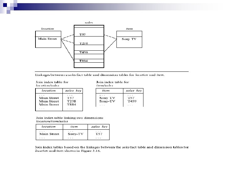
The join indexing method gained popularity from its use in relational database query processing. Traditional indexing maps the value in a given column to a list of rows having that value. In contrast, join indexing registers the joinable rows of two relations from a relational database. The star schema model of data warehouses makes join indexing attractive for cross table search, because the linkage between a fact table and its corresponding dimension tables comprises the foreign key of the fact table and the primary key of the dimension table. Join indexing maintains relationships between attribute values of a dimension (e. g. , within a dimension table) and the corresponding rows in the fact table. Join indices may span multiple dimensions to form composite join indices. We can use join indices to identify subcubes that are of interest.

4. 3. Efficient Processing of OLAP Queries The purpose of materializing cuboids and constructing OLAP index structures is to speed up query processing in data cubes. Given materialized views, query processing should proceed as follows: 1. Determine which operations should be performed on the available cuboids: This involves transforming any selection, projection, roll-up (groupby), and drill-down operations specified in the query into corresponding SQL and/or OLAP operations. For example, slicing and dicing a data cube may correspond to selection and/or projection operations on a materialized cuboid. 2. Determine to which materialized cuboid(s) the relevant operations should be applied: This involves identifying all of the materialized cuboids that may potentially be used to answer the query, pruning the above set using knowledge of “dominance” relationships among the cuboids, estimating the costs of using the remaining materialized cuboids, and selecting the cuboid with the least cost.

Efficient Processing OLAP Queries n Determine which operations should be performed on the available cuboids ¨ Transform drill, roll, etc. into corresponding SQL and/or OLAP operations, e. g. , dice = selection + projection n Determine which materialized cuboid(s) should be selected for OLAP op. ¨ Let the query to be processed be on {brand, province_or_state} with the condition “year = 2004”, and there are 4 materialized cuboids available: 1) {year, item_name, city} 2) {year, brand, country} 3) {year, brand, province_or_state} 4) {item_name, province_or_state} where year = 2004 Which should be selected to process the query? n Explore indexing structures and compressed vs. dense array. Data structs in Concepts MOLAP Mining: 66 18 September 2020 and Techniques

Data Warehouse Usage n Three kinds of data warehouse applications ¨ Information processing n ¨ ¨ n 67 supports querying, basic statistical analysis, and reporting using crosstabs, tables, charts and graphs Analytical processing n multidimensional analysis of data warehouse data n supports basic OLAP operations, slice-dice, drilling, pivoting Data mining n knowledge discovery from hidden patterns n supports associations, constructing analytical models, performing classification and prediction, and presenting the mining results using visualization tools. Differences among the three tasks 18 September 2020 Data Mining: Concepts and Techniques

From On-Line Analytical Processing (OLAP) to On Line Analytical Mining (OLAM) n Why online analytical mining? ¨ High quality of data in data warehouses n DW contains integrated, consistent, cleaned data ¨ Available information processing structure surrounding data warehouses n ODBC, OLEDB, Web accessing, service facilities, reporting and OLAP tools ¨ OLAP-based exploratory data analysis n Mining with drilling, dicing, pivoting, etc. ¨ On-line selection of data mining functions n Integration and swapping of multiple mining functions, algorithms, and tasks

An OLAM System Architecture Mining query Mining result Layer 4 User Interface User GUI API OLAM Engine OLAP Engine Layer 3 OLAP/OLAM Data Cube API Layer 2 MDDB Meta Data Filtering&Integration Database API Filtering Layer 1 Databases Data cleaning Data integration Warehouse Data Repository