Data Mining Association Rules Advanced Concepts and Algorithms

Data Mining Association Rules: Advanced Concepts and Algorithms Lecture Notes for Chapter 7 Introduction to Data Mining by Tan, Steinbach, Kumar © Tan, Steinbach, Kumar Introduction to Data Mining 4/18/2004 1

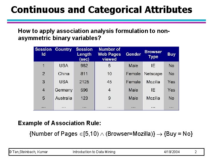
Continuous and Categorical Attributes How to apply association analysis formulation to nonasymmetric binary variables? Example of Association Rule: {Number of Pages [5, 10) (Browser=Mozilla)} {Buy = No} © Tan, Steinbach, Kumar Introduction to Data Mining 4/18/2004 2

Handling Categorical Attributes l Transform categorical attribute into asymmetric binary variables l Introduce a new “item” for each distinct attributevalue pair – Example: replace Browser Type attribute with u Browser Type = Internet Explorer u Browser Type = Mozilla © Tan, Steinbach, Kumar Introduction to Data Mining 4/18/2004 3

Handling Categorical Attributes l Potential Issues – What if attribute has many possible values Example: attribute country has more than 200 possible values u u Many of the attribute values may have very low support – Potential solution: Aggregate the low-support attribute values – What if distribution of attribute values is highly skewed u Example: 95% of the visitors have Buy = No u Most of the items will be associated with (Buy=No) item – Potential solution: drop the highly frequent items © Tan, Steinbach, Kumar Introduction to Data Mining 4/18/2004 4

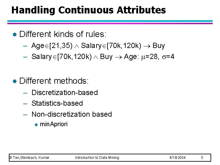
Handling Continuous Attributes l Different kinds of rules: – Age [21, 35) Salary [70 k, 120 k) Buy – Salary [70 k, 120 k) Buy Age: =28, =4 l Different methods: – Discretization-based – Statistics-based – Non-discretization based u min. Apriori © Tan, Steinbach, Kumar Introduction to Data Mining 4/18/2004 5

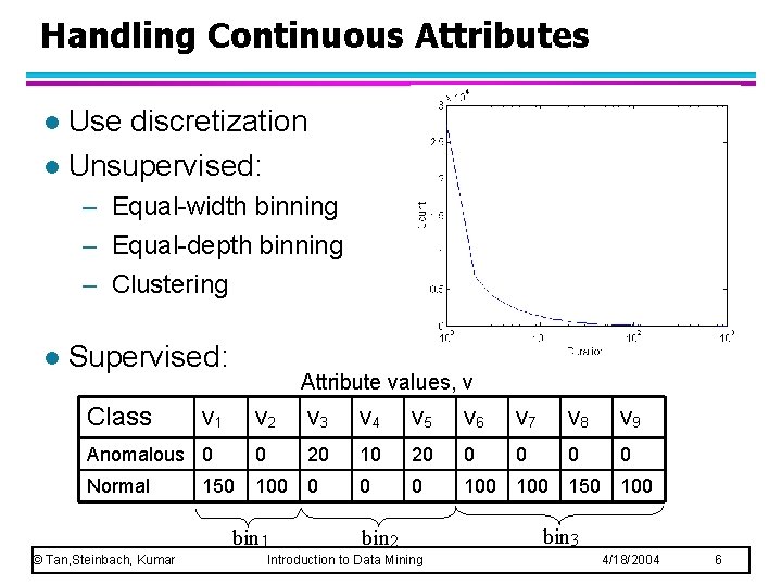
Handling Continuous Attributes Use discretization l Unsupervised: l – Equal-width binning – Equal-depth binning – Clustering l Supervised: Class Attribute values, v v 1 v 2 v 3 v 4 v 5 v 6 v 7 v 8 v 9 Anomalous 0 0 20 10 20 0 0 Normal 100 0 100 150 bin 1 © Tan, Steinbach, Kumar bin 2 Introduction to Data Mining bin 3 4/18/2004 6

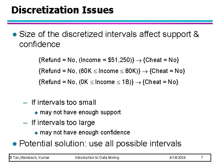
Discretization Issues l Size of the discretized intervals affect support & confidence {Refund = No, (Income = $51, 250)} {Cheat = No} {Refund = No, (60 K Income 80 K)} {Cheat = No} {Refund = No, (0 K Income 1 B)} {Cheat = No} – If intervals too small u may not have enough support – If intervals too large u l may not have enough confidence Potential solution: use all possible intervals © Tan, Steinbach, Kumar Introduction to Data Mining 4/18/2004 7

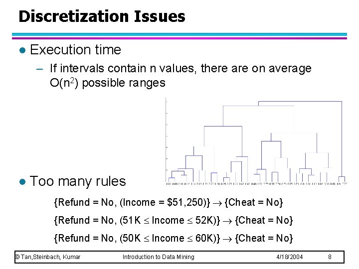
Discretization Issues l Execution time – If intervals contain n values, there are on average O(n 2) possible ranges l Too many rules {Refund = No, (Income = $51, 250)} {Cheat = No} {Refund = No, (51 K Income 52 K)} {Cheat = No} {Refund = No, (50 K Income 60 K)} {Cheat = No} © Tan, Steinbach, Kumar Introduction to Data Mining 4/18/2004 8

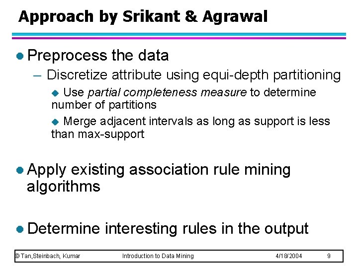
Approach by Srikant & Agrawal l Preprocess the data – Discretize attribute using equi-depth partitioning Use partial completeness measure to determine number of partitions u Merge adjacent intervals as long as support is less than max-support u l Apply existing association rule mining algorithms l Determine © Tan, Steinbach, Kumar interesting rules in the output Introduction to Data Mining 4/18/2004 9

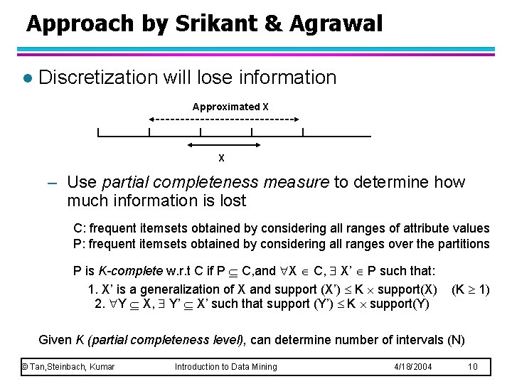
Approach by Srikant & Agrawal l Discretization will lose information Approximated X X – Use partial completeness measure to determine how much information is lost C: frequent itemsets obtained by considering all ranges of attribute values P: frequent itemsets obtained by considering all ranges over the partitions P is K-complete w. r. t C if P C, and X C, X’ P such that: 1. X’ is a generalization of X and support (X’) K support(X) 2. Y X, Y’ X’ such that support (Y’) K support(Y) (K 1) Given K (partial completeness level), can determine number of intervals (N) © Tan, Steinbach, Kumar Introduction to Data Mining 4/18/2004 10

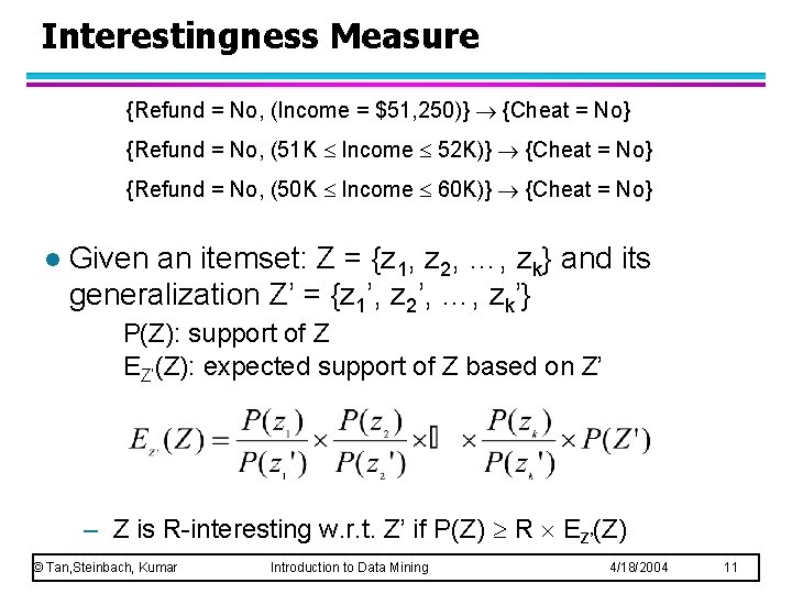
Interestingness Measure {Refund = No, (Income = $51, 250)} {Cheat = No} {Refund = No, (51 K Income 52 K)} {Cheat = No} {Refund = No, (50 K Income 60 K)} {Cheat = No} l Given an itemset: Z = {z 1, z 2, …, zk} and its generalization Z’ = {z 1’, z 2’, …, zk’} P(Z): support of Z EZ’(Z): expected support of Z based on Z’ – Z is R-interesting w. r. t. Z’ if P(Z) R EZ’(Z) © Tan, Steinbach, Kumar Introduction to Data Mining 4/18/2004 11

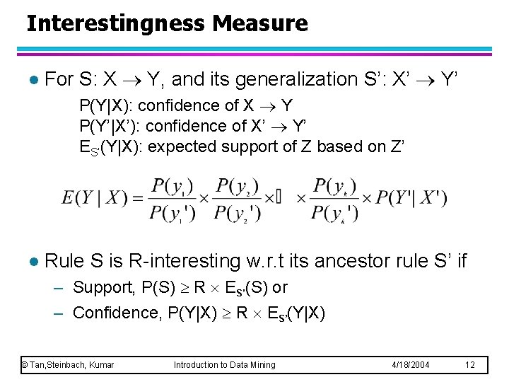
Interestingness Measure l For S: X Y, and its generalization S’: X’ Y’ P(Y|X): confidence of X Y P(Y’|X’): confidence of X’ Y’ ES’(Y|X): expected support of Z based on Z’ l Rule S is R-interesting w. r. t its ancestor rule S’ if – Support, P(S) R ES’(S) or – Confidence, P(Y|X) R ES’(Y|X) © Tan, Steinbach, Kumar Introduction to Data Mining 4/18/2004 12

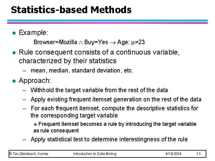
Statistics-based Methods l Example: Browser=Mozilla Buy=Yes Age: =23 l Rule consequent consists of a continuous variable, characterized by their statistics – mean, median, standard deviation, etc. l Approach: – Withhold the target variable from the rest of the data – Apply existing frequent itemset generation on the rest of the data – For each frequent itemset, compute the descriptive statistics for the corresponding target variable Frequent itemset becomes a rule by introducing the target variable as rule consequent u – Apply statistical test to determine interestingness of the rule © Tan, Steinbach, Kumar Introduction to Data Mining 4/18/2004 13

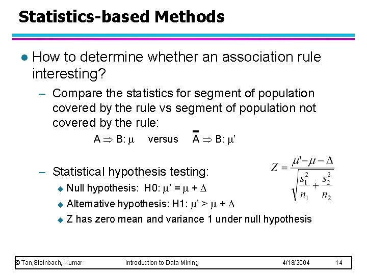
Statistics-based Methods l How to determine whether an association rule interesting? – Compare the statistics for segment of population covered by the rule vs segment of population not covered by the rule: A B: versus A B: ’ – Statistical hypothesis testing: u Null hypothesis: H 0: ’ = + u Alternative hypothesis: H 1: ’ > + u Z has zero mean and variance 1 under null hypothesis © Tan, Steinbach, Kumar Introduction to Data Mining 4/18/2004 14

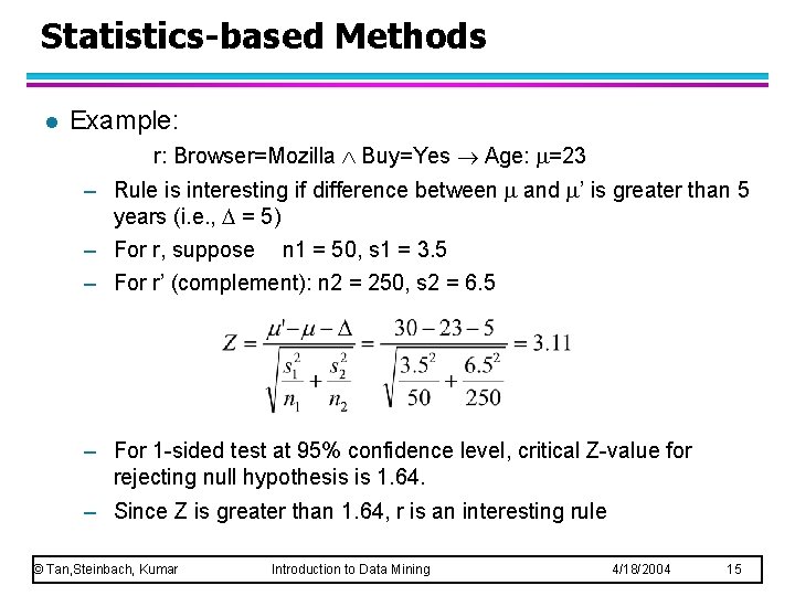
Statistics-based Methods l Example: r: Browser=Mozilla Buy=Yes Age: =23 – Rule is interesting if difference between and ’ is greater than 5 years (i. e. , = 5) – For r, suppose n 1 = 50, s 1 = 3. 5 – For r’ (complement): n 2 = 250, s 2 = 6. 5 – For 1 -sided test at 95% confidence level, critical Z-value for rejecting null hypothesis is 1. 64. – Since Z is greater than 1. 64, r is an interesting rule © Tan, Steinbach, Kumar Introduction to Data Mining 4/18/2004 15

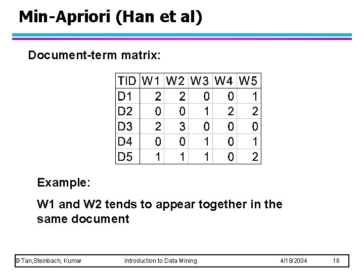
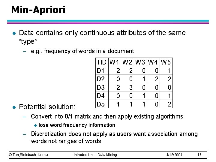
Min-Apriori (Han et al) Document-term matrix: Example: W 1 and W 2 tends to appear together in the same document © Tan, Steinbach, Kumar Introduction to Data Mining 4/18/2004 16

Min-Apriori l Data contains only continuous attributes of the same “type” – e. g. , frequency of words in a document l Potential solution: – Convert into 0/1 matrix and then apply existing algorithms u lose word frequency information – Discretization does not apply as users want association among words not ranges of words © Tan, Steinbach, Kumar Introduction to Data Mining 4/18/2004 17

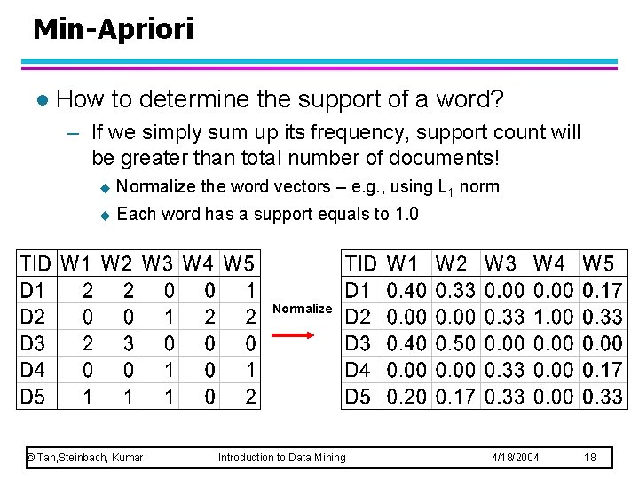
Min-Apriori l How to determine the support of a word? – If we simply sum up its frequency, support count will be greater than total number of documents! u Normalize the word vectors – e. g. , using L 1 norm u Each word has a support equals to 1. 0 Normalize © Tan, Steinbach, Kumar Introduction to Data Mining 4/18/2004 18

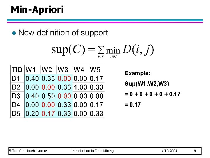
Min-Apriori l New definition of support: Example: Sup(W 1, W 2, W 3) = 0 + 0 + 0. 17 = 0. 17 © Tan, Steinbach, Kumar Introduction to Data Mining 4/18/2004 19

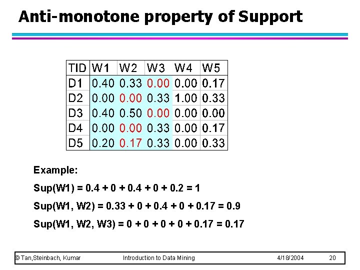
Anti-monotone property of Support Example: Sup(W 1) = 0. 4 + 0 + 0. 2 = 1 Sup(W 1, W 2) = 0. 33 + 0. 4 + 0. 17 = 0. 9 Sup(W 1, W 2, W 3) = 0 + 0 + 0. 17 = 0. 17 © Tan, Steinbach, Kumar Introduction to Data Mining 4/18/2004 20

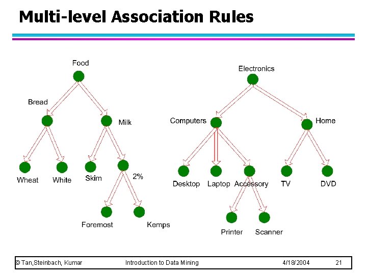
Multi-level Association Rules © Tan, Steinbach, Kumar Introduction to Data Mining 4/18/2004 21

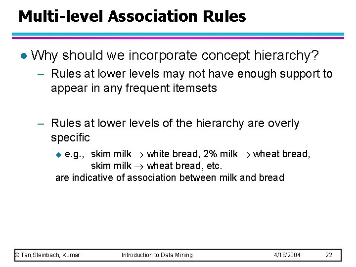
Multi-level Association Rules l Why should we incorporate concept hierarchy? – Rules at lower levels may not have enough support to appear in any frequent itemsets – Rules at lower levels of the hierarchy are overly specific e. g. , skim milk white bread, 2% milk wheat bread, skim milk wheat bread, etc. are indicative of association between milk and bread u © Tan, Steinbach, Kumar Introduction to Data Mining 4/18/2004 22

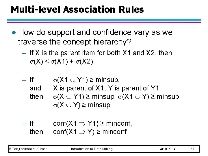
Multi-level Association Rules l How do support and confidence vary as we traverse the concept hierarchy? – If X is the parent item for both X 1 and X 2, then (X) ≤ (X 1) + (X 2) – If and then (X 1 Y 1) ≥ minsup, X is parent of X 1, Y is parent of Y 1 (X Y 1) ≥ minsup, (X 1 Y) ≥ minsup (X Y) ≥ minsup – If then conf(X 1 Y 1) ≥ minconf, conf(X 1 Y) ≥ minconf © Tan, Steinbach, Kumar Introduction to Data Mining 4/18/2004 23

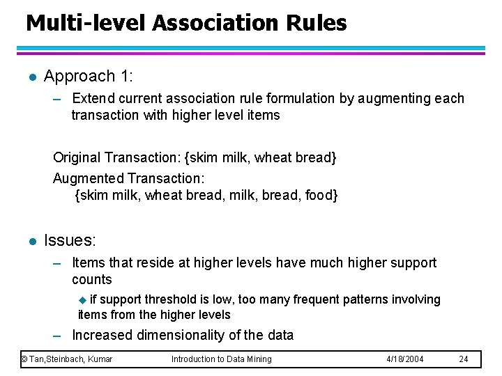
Multi-level Association Rules l Approach 1: – Extend current association rule formulation by augmenting each transaction with higher level items Original Transaction: {skim milk, wheat bread} Augmented Transaction: {skim milk, wheat bread, milk, bread, food} l Issues: – Items that reside at higher levels have much higher support counts if support threshold is low, too many frequent patterns involving items from the higher levels u – Increased dimensionality of the data © Tan, Steinbach, Kumar Introduction to Data Mining 4/18/2004 24

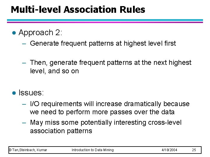
Multi-level Association Rules l Approach 2: – Generate frequent patterns at highest level first – Then, generate frequent patterns at the next highest level, and so on l Issues: – I/O requirements will increase dramatically because we need to perform more passes over the data – May miss some potentially interesting cross-level association patterns © Tan, Steinbach, Kumar Introduction to Data Mining 4/18/2004 25

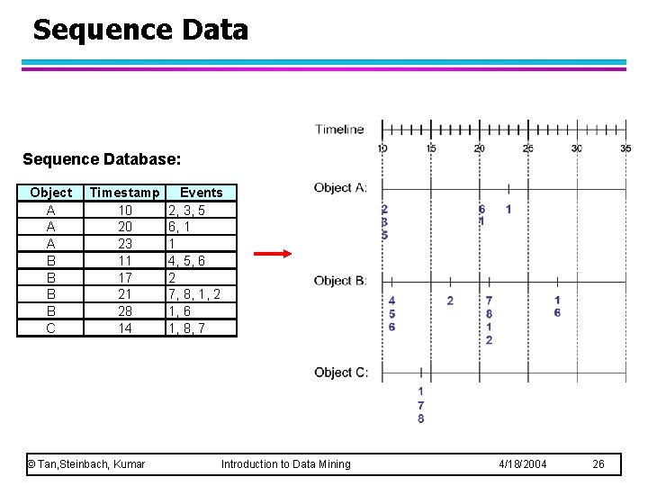
Sequence Database: Object A A A B B C Timestamp 10 20 23 11 17 21 28 14 © Tan, Steinbach, Kumar Events 2, 3, 5 6, 1 1 4, 5, 6 2 7, 8, 1, 2 1, 6 1, 8, 7 Introduction to Data Mining 4/18/2004 26

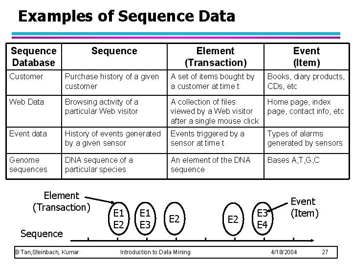
Examples of Sequence Database Sequence Element (Transaction) Event (Item) Customer Purchase history of a given customer A set of items bought by a customer at time t Books, diary products, CDs, etc Web Data Browsing activity of a particular Web visitor A collection of files viewed by a Web visitor after a single mouse click Home page, index page, contact info, etc Event data History of events generated by a given sensor Events triggered by a sensor at time t Types of alarms generated by sensors Genome sequences DNA sequence of a particular species An element of the DNA sequence Bases A, T, G, C Element (Transaction) Sequence © Tan, Steinbach, Kumar E 1 E 2 E 1 E 3 E 2 Introduction to Data Mining E 2 E 3 E 4 Event (Item) 4/18/2004 27

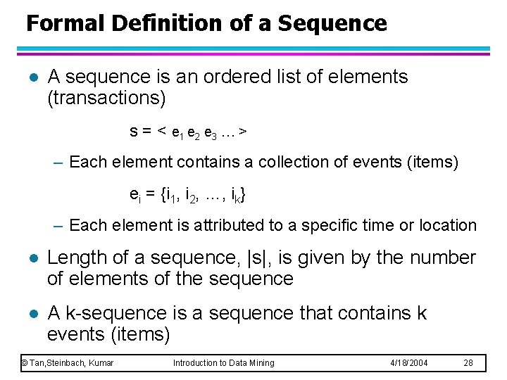
Formal Definition of a Sequence l A sequence is an ordered list of elements (transactions) s = < e 1 e 2 e 3 … > – Each element contains a collection of events (items) ei = {i 1, i 2, …, ik} – Each element is attributed to a specific time or location l Length of a sequence, |s|, is given by the number of elements of the sequence l A k-sequence is a sequence that contains k events (items) © Tan, Steinbach, Kumar Introduction to Data Mining 4/18/2004 28

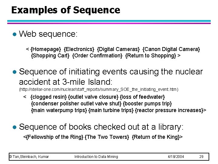
Examples of Sequence l Web sequence: < {Homepage} {Electronics} {Digital Cameras} {Canon Digital Camera} {Shopping Cart} {Order Confirmation} {Return to Shopping} > l Sequence of initiating events causing the nuclear accident at 3 -mile Island: (http: //stellar-one. com/nuclear/staff_reports/summary_SOE_the_initiating_event. htm) < {clogged resin} {outlet valve closure} {loss of feedwater} {condenser polisher outlet valve shut} {booster pumps trip} {main waterpump trips} {main turbine trips} {reactor pressure increases}> l Sequence of books checked out at a library: <{Fellowship of the Ring} {The Two Towers} {Return of the King}> © Tan, Steinbach, Kumar Introduction to Data Mining 4/18/2004 29

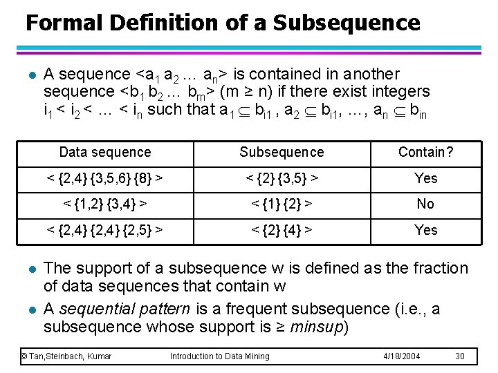
Formal Definition of a Subsequence l l l A sequence <a 1 a 2 … an> is contained in another sequence <b 1 b 2 … bm> (m ≥ n) if there exist integers i 1 < i 2 < … < in such that a 1 bi 1 , a 2 bi 1, …, an bin Data sequence Subsequence Contain? < {2, 4} {3, 5, 6} {8} > < {2} {3, 5} > Yes < {1, 2} {3, 4} > < {1} {2} > No < {2, 4} {2, 5} > < {2} {4} > Yes The support of a subsequence w is defined as the fraction of data sequences that contain w A sequential pattern is a frequent subsequence (i. e. , a subsequence whose support is ≥ minsup) © Tan, Steinbach, Kumar Introduction to Data Mining 4/18/2004 30

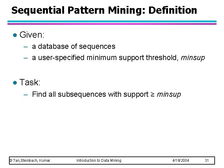
Sequential Pattern Mining: Definition l Given: – a database of sequences – a user-specified minimum support threshold, minsup l Task: – Find all subsequences with support ≥ minsup © Tan, Steinbach, Kumar Introduction to Data Mining 4/18/2004 31

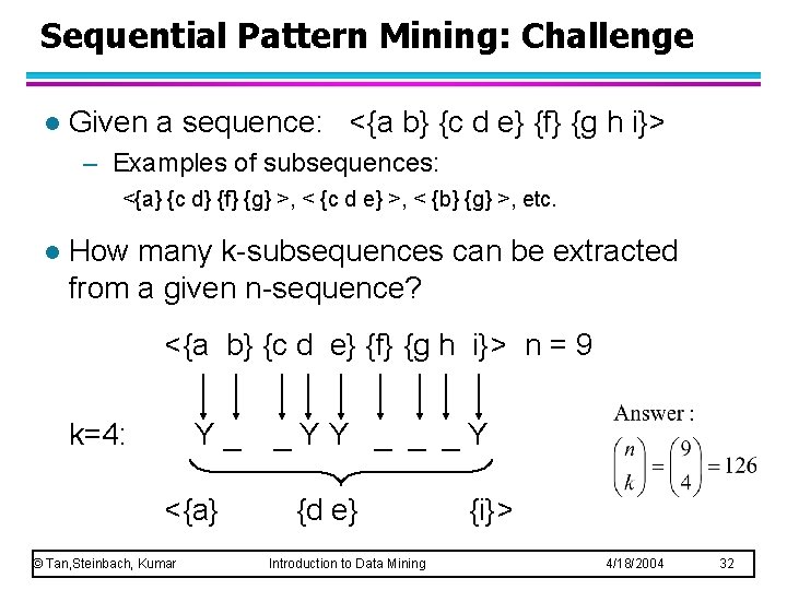
Sequential Pattern Mining: Challenge l Given a sequence: <{a b} {c d e} {f} {g h i}> – Examples of subsequences: <{a} {c d} {f} {g} >, < {c d e} >, < {b} {g} >, etc. l How many k-subsequences can be extracted from a given n-sequence? <{a b} {c d e} {f} {g h i}> n = 9 k=4: Y_ <{a} © Tan, Steinbach, Kumar _YY _ _ _Y {d e} Introduction to Data Mining {i}> 4/18/2004 32

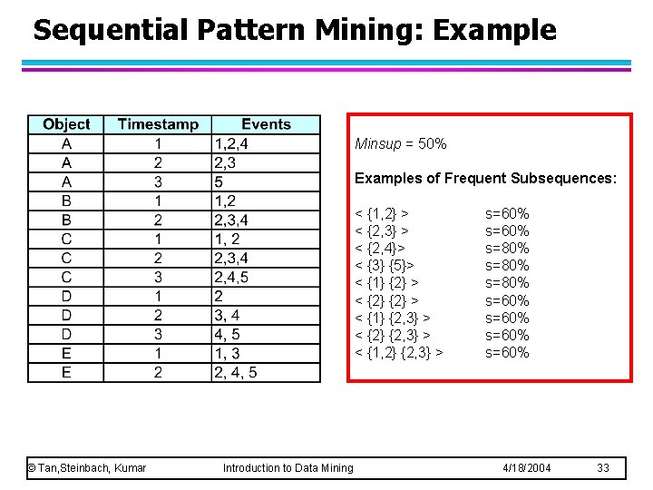
Sequential Pattern Mining: Example Minsup = 50% Examples of Frequent Subsequences: < {1, 2} > < {2, 3} > < {2, 4}> < {3} {5}> < {1} {2} > < {1} {2, 3} > < {2} {2, 3} > < {1, 2} {2, 3} > © Tan, Steinbach, Kumar Introduction to Data Mining s=60% s=80% s=60% 4/18/2004 33

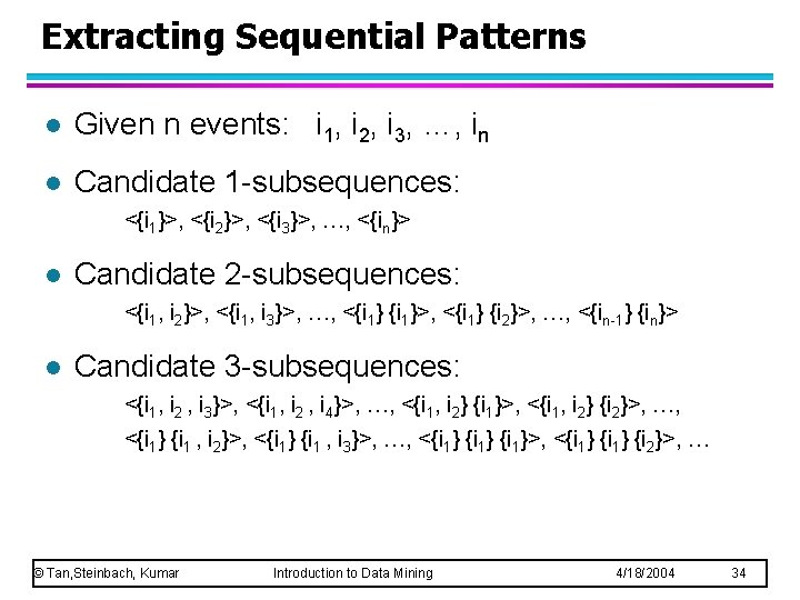
Extracting Sequential Patterns l Given n events: i 1, i 2, i 3, …, in l Candidate 1 -subsequences: <{i 1}>, <{i 2}>, <{i 3}>, …, <{in}> l Candidate 2 -subsequences: <{i 1, i 2}>, <{i 1, i 3}>, …, <{i 1}>, <{i 1} {i 2}>, …, <{in-1} {in}> l Candidate 3 -subsequences: <{i 1, i 2 , i 3}>, <{i 1, i 2 , i 4}>, …, <{i 1, i 2} {i 1}>, <{i 1, i 2} {i 2}>, …, <{i 1} {i 1 , i 2}>, <{i 1} {i 1 , i 3}>, …, <{i 1}>, <{i 1} {i 2}>, … © Tan, Steinbach, Kumar Introduction to Data Mining 4/18/2004 34

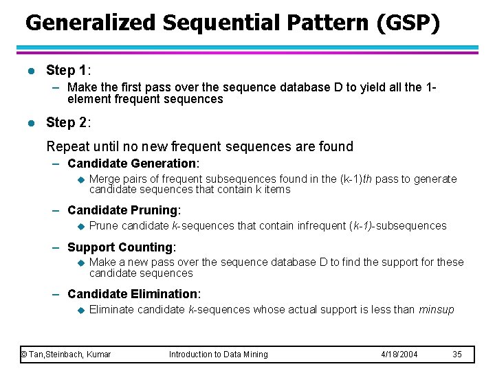
Generalized Sequential Pattern (GSP) l Step 1: – Make the first pass over the sequence database D to yield all the 1 element frequent sequences l Step 2: Repeat until no new frequent sequences are found – Candidate Generation: u Merge pairs of frequent subsequences found in the (k-1)th pass to generate candidate sequences that contain k items – Candidate Pruning: u Prune candidate k-sequences that contain infrequent (k-1)-subsequences – Support Counting: u Make a new pass over the sequence database D to find the support for these candidate sequences – Candidate Elimination: u Eliminate candidate k-sequences whose actual support is less than minsup © Tan, Steinbach, Kumar Introduction to Data Mining 4/18/2004 35

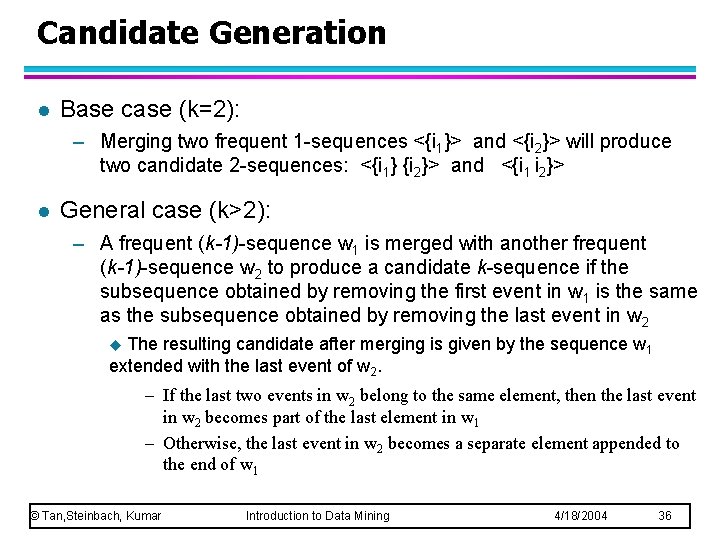
Candidate Generation l Base case (k=2): – Merging two frequent 1 -sequences <{i 1}> and <{i 2}> will produce two candidate 2 -sequences: <{i 1} {i 2}> and <{i 1 i 2}> l General case (k>2): – A frequent (k-1)-sequence w 1 is merged with another frequent (k-1)-sequence w 2 to produce a candidate k-sequence if the subsequence obtained by removing the first event in w 1 is the same as the subsequence obtained by removing the last event in w 2 The resulting candidate after merging is given by the sequence w 1 extended with the last event of w 2. u – If the last two events in w 2 belong to the same element, then the last event in w 2 becomes part of the last element in w 1 – Otherwise, the last event in w 2 becomes a separate element appended to the end of w 1 © Tan, Steinbach, Kumar Introduction to Data Mining 4/18/2004 36

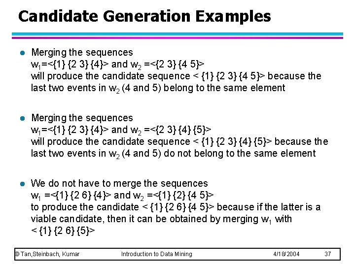
Candidate Generation Examples l Merging the sequences w 1=<{1} {2 3} {4}> and w 2 =<{2 3} {4 5}> will produce the candidate sequence < {1} {2 3} {4 5}> because the last two events in w 2 (4 and 5) belong to the same element l Merging the sequences w 1=<{1} {2 3} {4}> and w 2 =<{2 3} {4} {5}> will produce the candidate sequence < {1} {2 3} {4} {5}> because the last two events in w 2 (4 and 5) do not belong to the same element l We do not have to merge the sequences w 1 =<{1} {2 6} {4}> and w 2 =<{1} {2} {4 5}> to produce the candidate < {1} {2 6} {4 5}> because if the latter is a viable candidate, then it can be obtained by merging w 1 with < {1} {2 6} {5}> © Tan, Steinbach, Kumar Introduction to Data Mining 4/18/2004 37

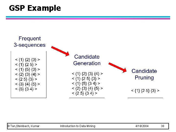
GSP Example © Tan, Steinbach, Kumar Introduction to Data Mining 4/18/2004 38

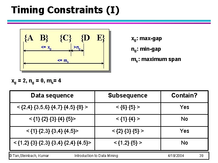
Timing Constraints (I) {A B} {C} <= xg {D E} xg: max-gap >ng ng: min-gap ms: maximum span <= ms xg = 2, ng = 0, ms= 4 Data sequence Subsequence Contain? < {2, 4} {3, 5, 6} {4, 7} {4, 5} {8} > < {6} {5} > Yes < {1} {2} {3} {4} {5}> < {1} {4} > No < {1} {2, 3} {3, 4} {4, 5}> < {2} {3} {5} > Yes < {1, 2} {3} {2, 3} {3, 4} {2, 4} {4, 5}> < {1, 2} {5} > No © Tan, Steinbach, Kumar Introduction to Data Mining 4/18/2004 39

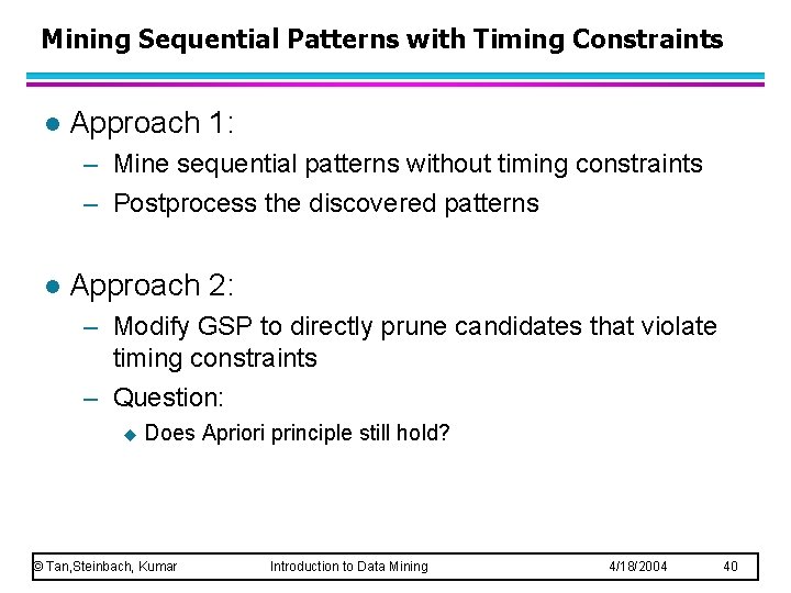
Mining Sequential Patterns with Timing Constraints l Approach 1: – Mine sequential patterns without timing constraints – Postprocess the discovered patterns l Approach 2: – Modify GSP to directly prune candidates that violate timing constraints – Question: u Does Apriori principle still hold? © Tan, Steinbach, Kumar Introduction to Data Mining 4/18/2004 40

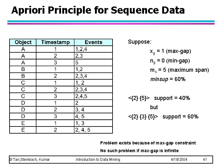
Apriori Principle for Sequence Data Suppose: xg = 1 (max-gap) ng = 0 (min-gap) ms = 5 (maximum span) minsup = 60% <{2} {5}> support = 40% but <{2} {3} {5}> support = 60% Problem exists because of max-gap constraint No such problem if max-gap is infinite © Tan, Steinbach, Kumar Introduction to Data Mining 4/18/2004 41

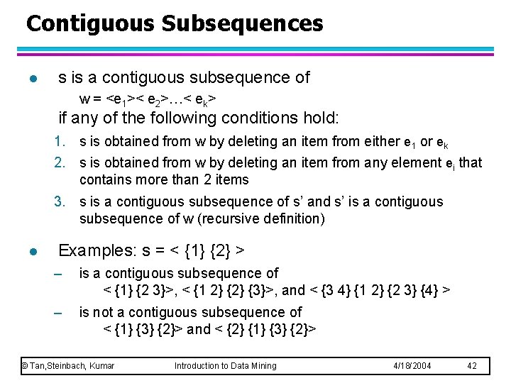
Contiguous Subsequences l s is a contiguous subsequence of w = <e 1>< e 2>…< ek> if any of the following conditions hold: 1. s is obtained from w by deleting an item from either e 1 or ek 2. s is obtained from w by deleting an item from any element ei that contains more than 2 items 3. s is a contiguous subsequence of s’ and s’ is a contiguous subsequence of w (recursive definition) l Examples: s = < {1} {2} > – is a contiguous subsequence of < {1} {2 3}>, < {1 2} {3}>, and < {3 4} {1 2} {2 3} {4} > – is not a contiguous subsequence of < {1} {3} {2}> and < {2} {1} {3} {2}> © Tan, Steinbach, Kumar Introduction to Data Mining 4/18/2004 42

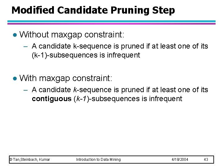
Modified Candidate Pruning Step l Without maxgap constraint: – A candidate k-sequence is pruned if at least one of its (k-1)-subsequences is infrequent l With maxgap constraint: – A candidate k-sequence is pruned if at least one of its contiguous (k-1)-subsequences is infrequent © Tan, Steinbach, Kumar Introduction to Data Mining 4/18/2004 43

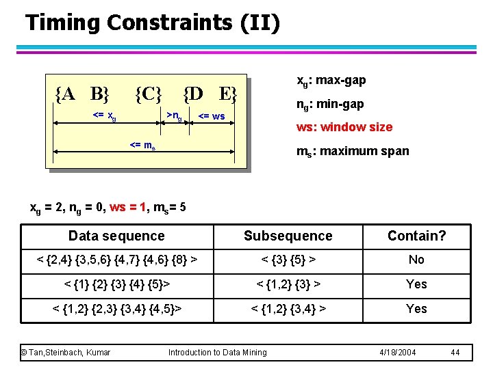
Timing Constraints (II) {A B} {C} <= xg xg: max-gap {D E} >ng ng: min-gap <= ws ws: window size <= ms ms: maximum span xg = 2, ng = 0, ws = 1, ms= 5 Data sequence Subsequence Contain? < {2, 4} {3, 5, 6} {4, 7} {4, 6} {8} > < {3} {5} > No < {1} {2} {3} {4} {5}> < {1, 2} {3} > Yes < {1, 2} {2, 3} {3, 4} {4, 5}> < {1, 2} {3, 4} > Yes © Tan, Steinbach, Kumar Introduction to Data Mining 4/18/2004 44

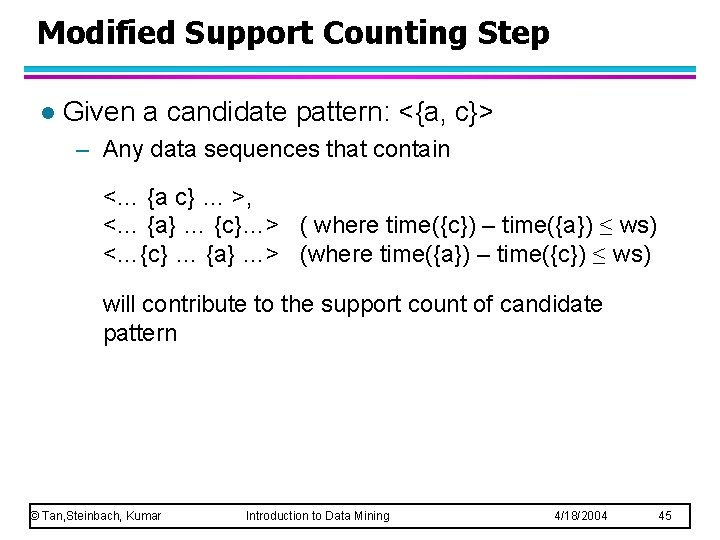
Modified Support Counting Step l Given a candidate pattern: <{a, c}> – Any data sequences that contain <… {a c} … >, <… {a} … {c}…> ( where time({c}) – time({a}) ≤ ws) <…{c} … {a} …> (where time({a}) – time({c}) ≤ ws) will contribute to the support count of candidate pattern © Tan, Steinbach, Kumar Introduction to Data Mining 4/18/2004 45

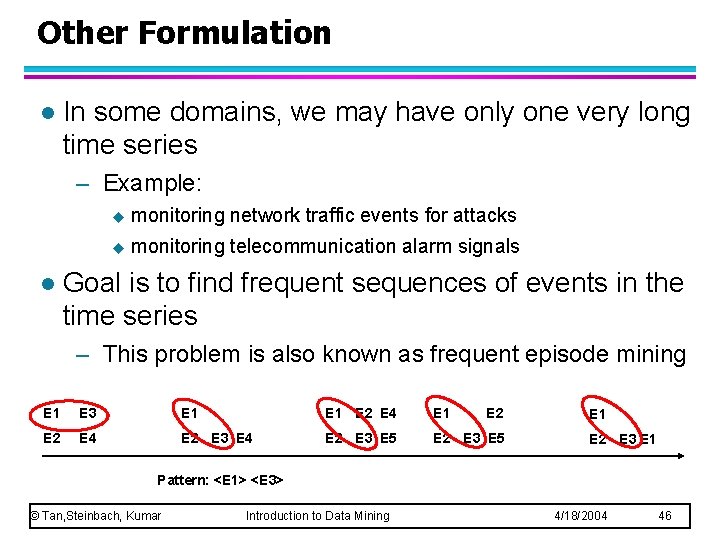
Other Formulation l In some domains, we may have only one very long time series – Example: l u monitoring network traffic events for attacks u monitoring telecommunication alarm signals Goal is to find frequent sequences of events in the time series – This problem is also known as frequent episode mining E 1 E 3 E 1 E 2 E 4 E 2 E 3 E 5 E 1 E 2 E 3 E 1 Pattern: <E 1> <E 3> © Tan, Steinbach, Kumar Introduction to Data Mining 4/18/2004 46

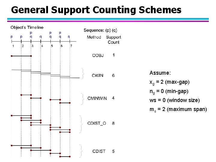
General Support Counting Schemes Assume: xg = 2 (max-gap) ng = 0 (min-gap) ws = 0 (window size) ms = 2 (maximum span)

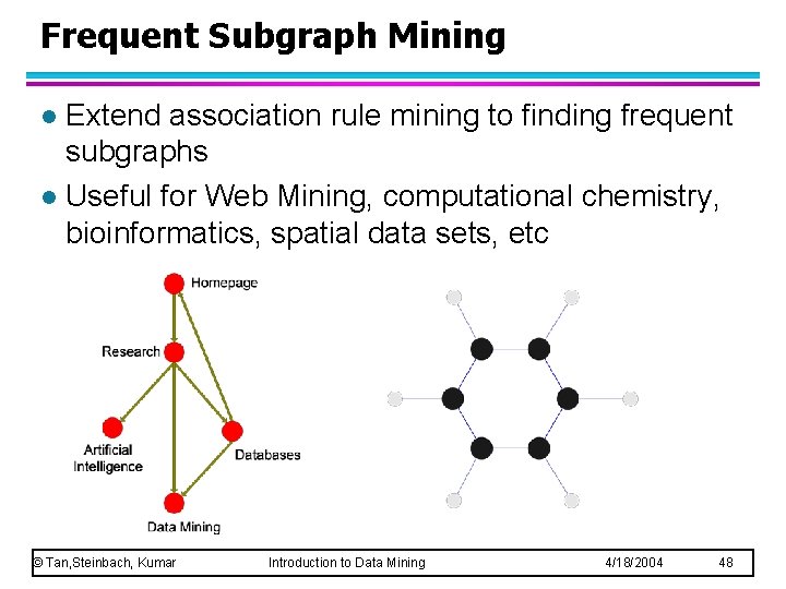
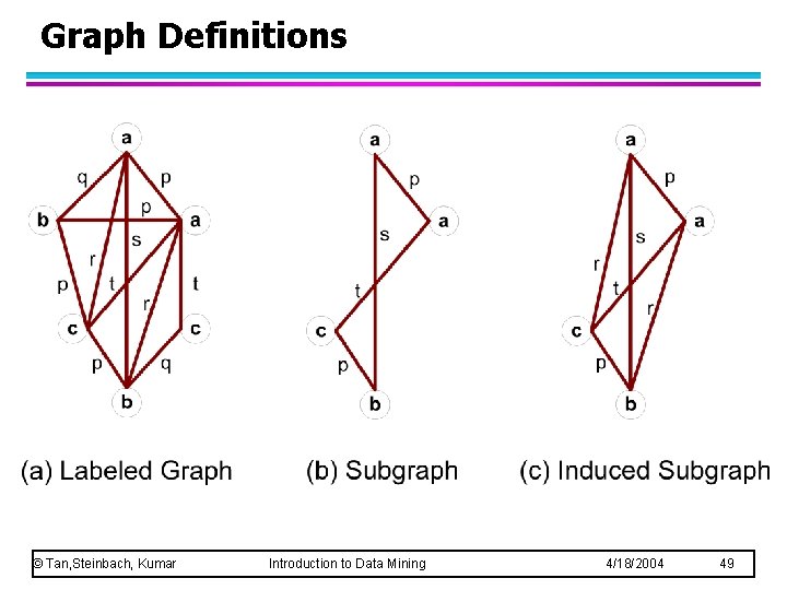
Frequent Subgraph Mining Extend association rule mining to finding frequent subgraphs l Useful for Web Mining, computational chemistry, bioinformatics, spatial data sets, etc l © Tan, Steinbach, Kumar Introduction to Data Mining 4/18/2004 48

Graph Definitions © Tan, Steinbach, Kumar Introduction to Data Mining 4/18/2004 49

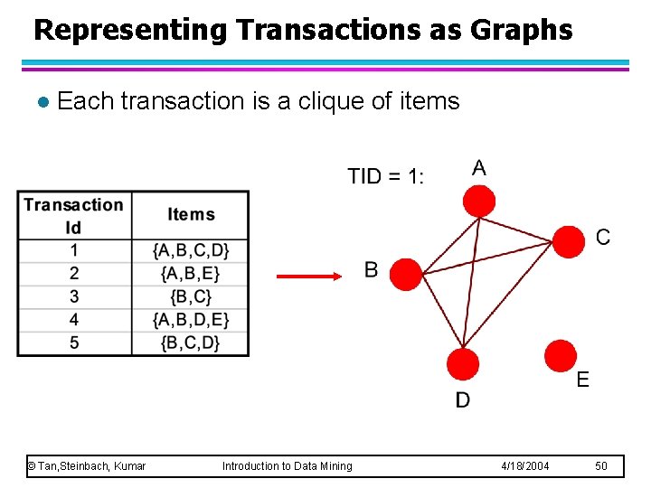
Representing Transactions as Graphs l Each transaction is a clique of items © Tan, Steinbach, Kumar Introduction to Data Mining 4/18/2004 50

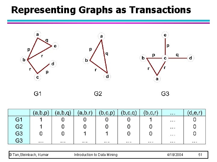
Representing Graphs as Transactions © Tan, Steinbach, Kumar Introduction to Data Mining 4/18/2004 51

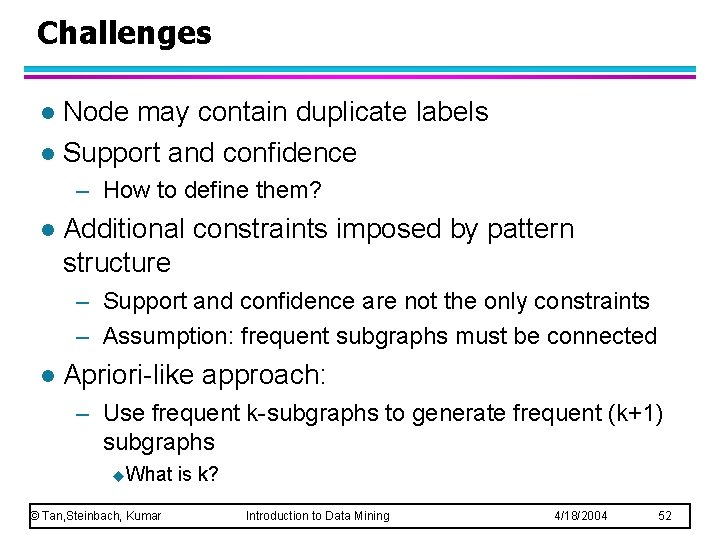
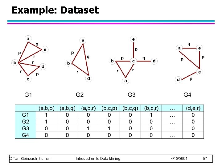
Challenges Node may contain duplicate labels l Support and confidence l – How to define them? l Additional constraints imposed by pattern structure – Support and confidence are not the only constraints – Assumption: frequent subgraphs must be connected l Apriori-like approach: – Use frequent k-subgraphs to generate frequent (k+1) subgraphs u. What © Tan, Steinbach, Kumar is k? Introduction to Data Mining 4/18/2004 52

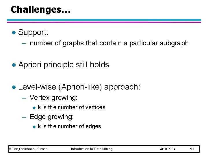
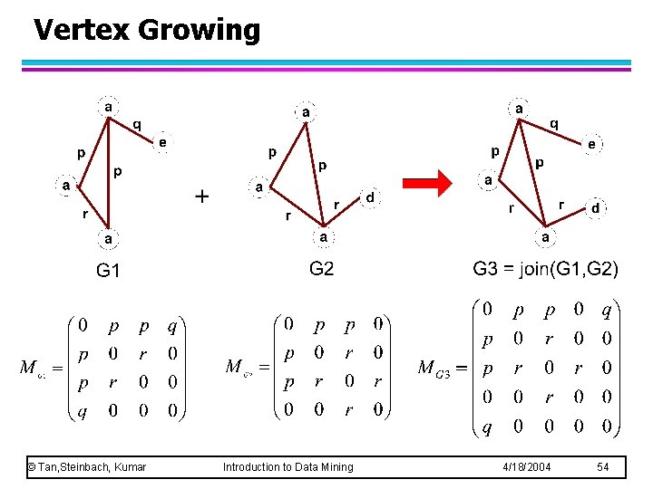
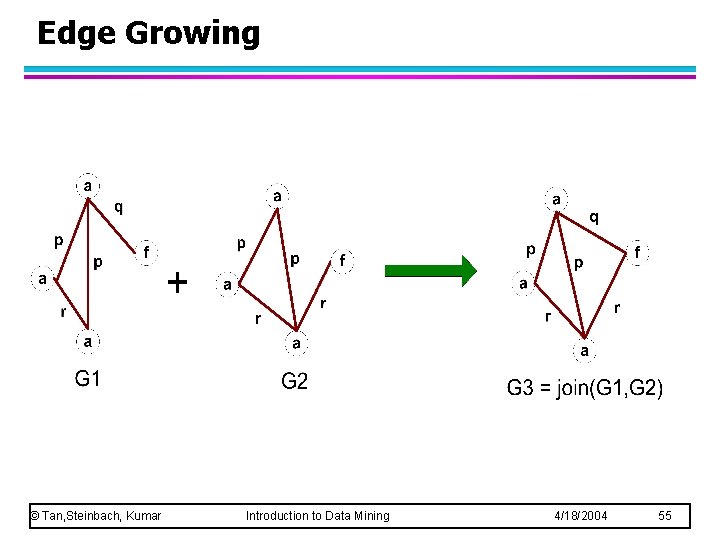
Challenges… l Support: – number of graphs that contain a particular subgraph l Apriori principle still holds l Level-wise (Apriori-like) approach: – Vertex growing: u k is the number of vertices – Edge growing: u k is the number of edges © Tan, Steinbach, Kumar Introduction to Data Mining 4/18/2004 53

Vertex Growing © Tan, Steinbach, Kumar Introduction to Data Mining 4/18/2004 54

Edge Growing © Tan, Steinbach, Kumar Introduction to Data Mining 4/18/2004 55

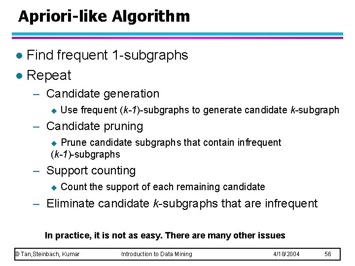
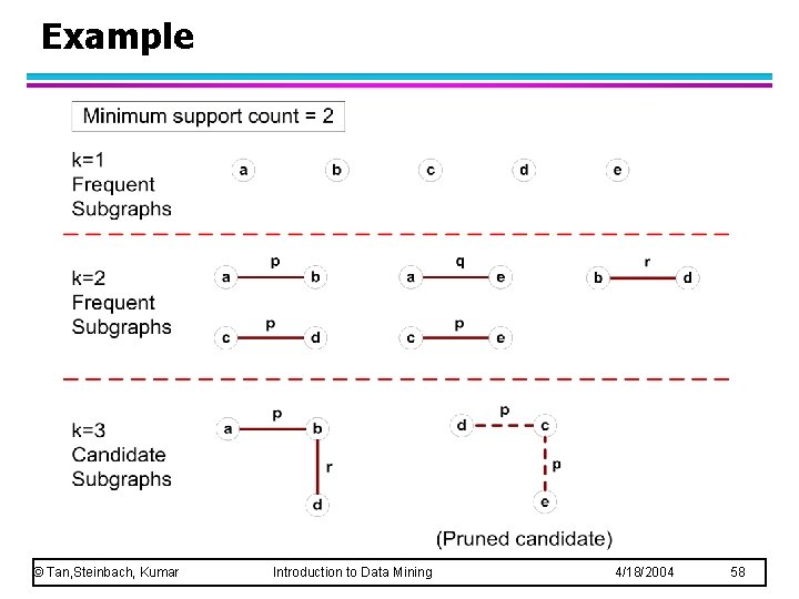
Apriori-like Algorithm Find frequent 1 -subgraphs l Repeat l – Candidate generation u Use frequent (k-1)-subgraphs to generate candidate k-subgraph – Candidate pruning Prune candidate subgraphs that contain infrequent (k-1)-subgraphs u – Support counting u Count the support of each remaining candidate – Eliminate candidate k-subgraphs that are infrequent In practice, it is not as easy. There are many other issues © Tan, Steinbach, Kumar Introduction to Data Mining 4/18/2004 56

Example: Dataset © Tan, Steinbach, Kumar Introduction to Data Mining 4/18/2004 57

Example © Tan, Steinbach, Kumar Introduction to Data Mining 4/18/2004 58

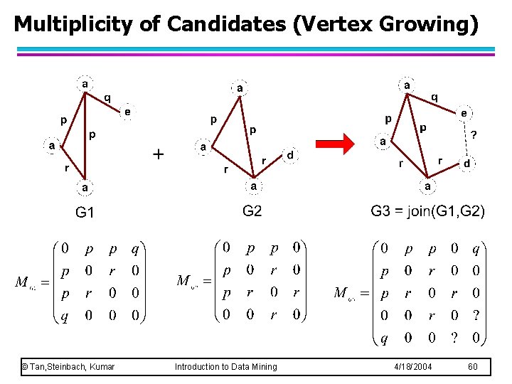
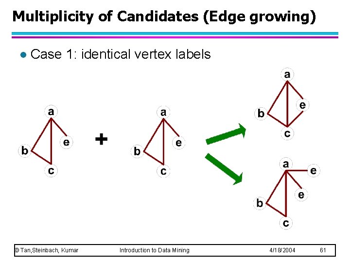
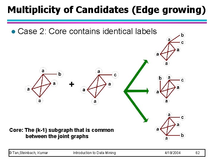
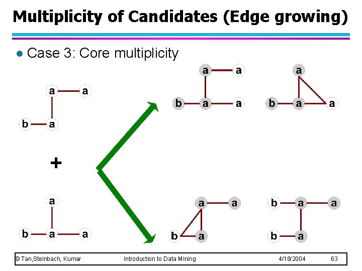
Candidate Generation l In Apriori: – Merging two frequent k-itemsets will produce a candidate (k+1)-itemset l In frequent subgraph mining (vertex/edge growing) – Merging two frequent k-subgraphs may produce more than one candidate (k+1)-subgraph © Tan, Steinbach, Kumar Introduction to Data Mining 4/18/2004 59

Multiplicity of Candidates (Vertex Growing) © Tan, Steinbach, Kumar Introduction to Data Mining 4/18/2004 60

Multiplicity of Candidates (Edge growing) l Case 1: identical vertex labels © Tan, Steinbach, Kumar Introduction to Data Mining 4/18/2004 61

Multiplicity of Candidates (Edge growing) l Case 2: Core contains identical labels Core: The (k-1) subgraph that is common between the joint graphs © Tan, Steinbach, Kumar Introduction to Data Mining 4/18/2004 62

Multiplicity of Candidates (Edge growing) l Case 3: Core multiplicity © Tan, Steinbach, Kumar Introduction to Data Mining 4/18/2004 63

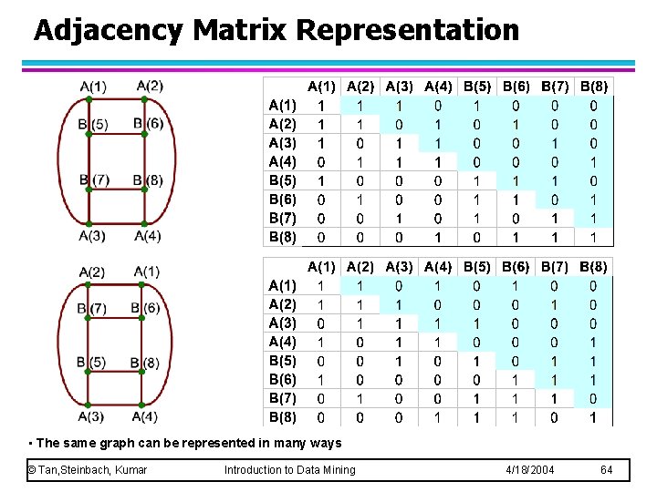
Adjacency Matrix Representation • The same graph can be represented in many ways © Tan, Steinbach, Kumar Introduction to Data Mining 4/18/2004 64

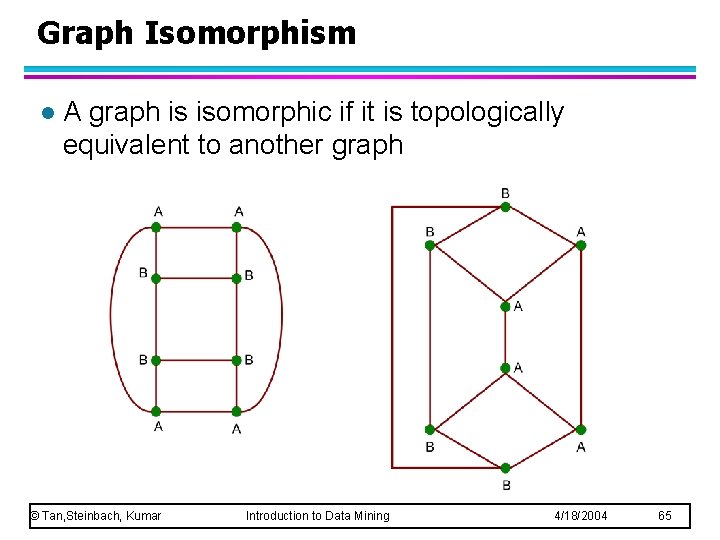
Graph Isomorphism l A graph is isomorphic if it is topologically equivalent to another graph © Tan, Steinbach, Kumar Introduction to Data Mining 4/18/2004 65

Graph Isomorphism l Test for graph isomorphism is needed: – During candidate generation step, to determine whether a candidate has been generated – During candidate pruning step, to check whether its (k-1)-subgraphs are frequent – During candidate counting, to check whether a candidate is contained within another graph © Tan, Steinbach, Kumar Introduction to Data Mining 4/18/2004 66

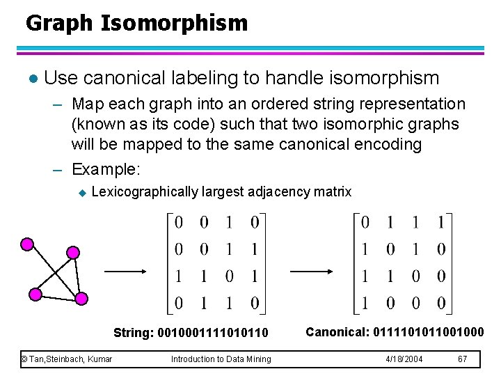
Graph Isomorphism l Use canonical labeling to handle isomorphism – Map each graph into an ordered string representation (known as its code) such that two isomorphic graphs will be mapped to the same canonical encoding – Example: u Lexicographically largest adjacency matrix String: 0010001111010110 © Tan, Steinbach, Kumar Introduction to Data Mining Canonical: 0111101011001000 4/18/2004 67