CS 412 Intro to Data Mining Chapter 5

CS 412 Intro. to Data Mining Chapter 5. Data Cube Technology Jiawei Han, Computer Science, Univ. Illinois at Urbana-Champaign, 2017 1

10/3/2020 2 Data Mining: Concepts and Techniques 2

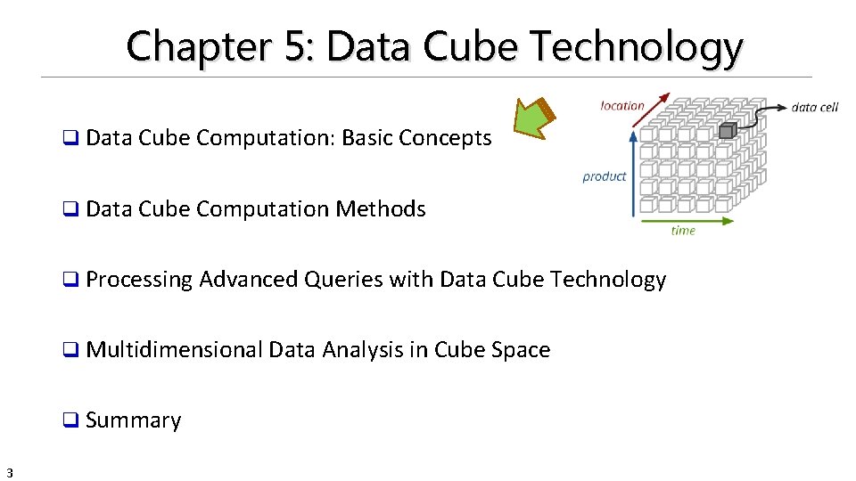
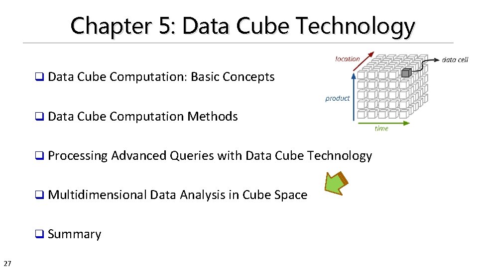
Chapter 5: Data Cube Technology q Data Cube Computation: Basic Concepts q Data Cube Computation Methods q Processing Advanced Queries with Data Cube Technology q Multidimensional Data Analysis in Cube Space q Summary 3

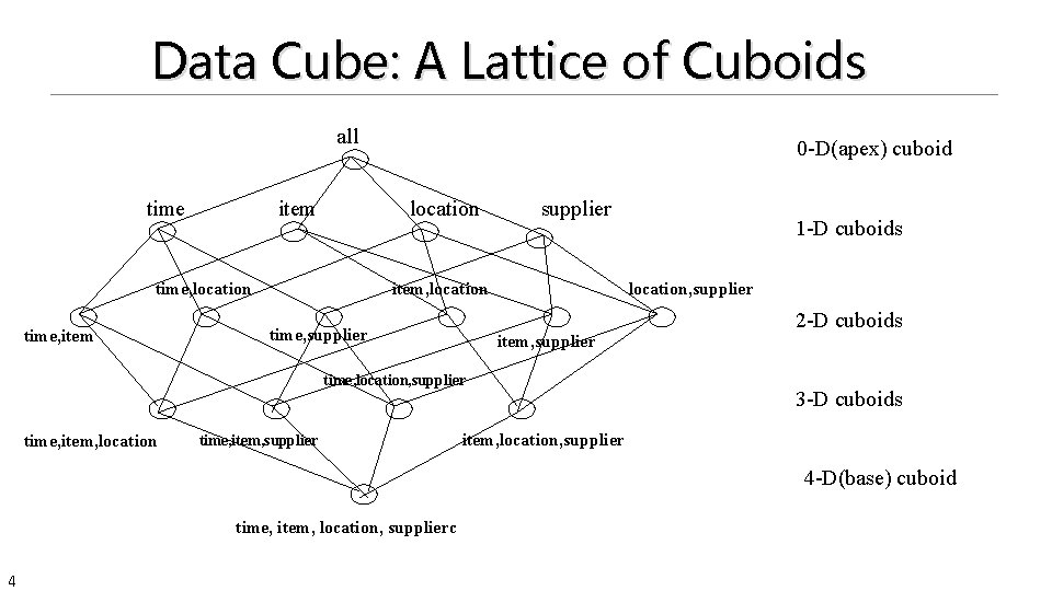
Data Cube: A Lattice of Cuboids all time item location time, item 0 -D(apex) cuboid supplier item, location time, supplier location, supplier item, supplier time, location, supplier time, item, location time, item, supplier 1 -D cuboids 2 -D cuboids 3 -D cuboids item, location, supplier 4 -D(base) cuboid time, item, location, supplierc 4

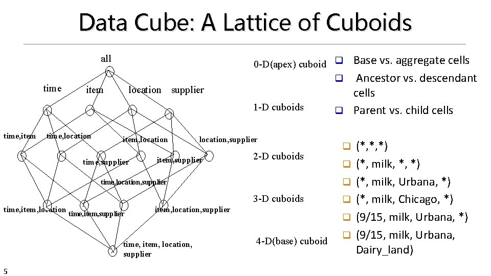
Data Cube: A Lattice of Cuboids all time item location supplier 1 -D cuboids time, item time, location item, location time, supplier location, supplier item, supplier 2 -D cuboids 3 -D cuboids time, item, supplier item, location, supplier time, item, location, supplier 5 q q q time, location, supplier time, item, location Base vs. aggregate cells Ancestor vs. descendant cells q Parent vs. child cells 0 -D(apex) cuboid q q 4 -D(base) cuboid q (*, *, *) (*, milk, Urbana, *) (*, milk, Chicago, *) (9/15, milk, Urbana, Dairy_land)

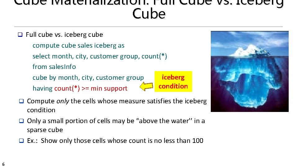
Cube Materialization: Full Cube vs. Iceberg Cube q Full cube vs. iceberg cube compute cube sales iceberg as select month, city, customer group, count(*) from sales. Info iceberg cube by month, city, customer group condition having count(*) >= min support Compute only the cells whose measure satisfies the iceberg condition q Only a small portion of cells may be “above the water’’ in a sparse cube q Ex. : Show only those cells whose count is no less than 100 q 6

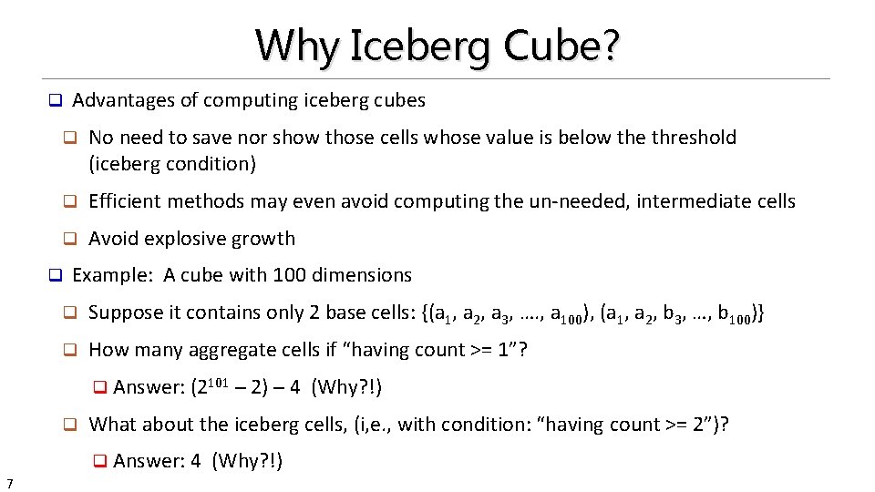
Why Iceberg Cube? q Advantages of computing iceberg cubes q No need to save nor show those cells whose value is below the threshold (iceberg condition) q Efficient methods may even avoid computing the un-needed, intermediate cells q Avoid explosive growth q Example: A cube with 100 dimensions q Suppose it contains only 2 base cells: {(a 1, a 2, a 3, …. , a 100), (a 1, a 2, b 3, …, b 100)} q How many aggregate cells if “having count >= 1”? q Answer: (2101 ─ 2) ─ 4 q What about the iceberg cells, (i, e. , with condition: “having count >= 2”)? q Answer: 4 7 (Why? !)

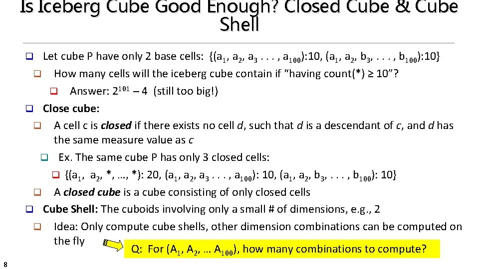
Is Iceberg Cube Good Enough? Closed Cube & Cube Shell Let cube P have only 2 base cells: {(a 1, a 2, a 3. . . , a 100): 10, (a 1, a 2, b 3, . . . , b 100): 10} q How many cells will the iceberg cube contain if “having count(*) ≥ 10”? q Answer: 2101 ─ 4 (still too big!) q Close cube: q A cell c is closed if there exists no cell d, such that d is a descendant of c, and d has the same measure value as c q Ex. The same cube P has only 3 closed cells: q {(a 1, a 2, *, …, *): 20, (a 1, a 2, a 3. . . , a 100): 10, (a 1, a 2, b 3, . . . , b 100): 10} q A closed cube is a cube consisting of only closed cells q Cube Shell: The cuboids involving only a small # of dimensions, e. g. , 2 q Idea: Only compute cube shells, other dimension combinations can be computed on the fly Q: For (A 1, A 2, … A 100), how many combinations to compute? q 8

Chapter 5: Data Cube Technology q Data Cube Computation: Basic Concepts q Data Cube Computation Methods q Processing Advanced Queries with Data Cube Technology q Multidimensional Data Analysis in Cube Space q Summary 9

Roadmap for Efficient Computation General computation heuristics (Agarwal et al. ’ 96) q Computing full/iceberg cubes: 3 methodologies q Bottom-Up: Multi-Way array aggregation (Zhao, Deshpande & Naughton, SIGMOD’ 97) q Top-down: q BUC (Beyer & Ramarkrishnan, SIGMOD’ 99) q Integrating Top-Down and Bottom-Up: q Star-cubing algorithm (Xin, Han, Li & Wah: VLDB’ 03) q High-dimensional OLAP: q A Shell-Fragment Approach (Li, et al. VLDB’ 04) q Computing alternative kinds of cubes: q Partial cube, closed cube, approximate cube, …… q 10

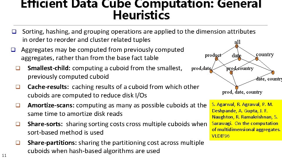
Efficient Data Cube Computation: General Heuristics Sorting, hashing, and grouping operations are applied to the dimension attributes in order to reorder and cluster related tuples all q Aggregates may be computed from previously computed country product date aggregates, rather than from the base fact table prod, date prod, country q Smallest-child: computing a cuboid from the smallest, previously computed cuboid date, country q Cache-results: caching results of a cuboid from which other prod, date, country cuboids are computed to reduce disk I/Os q Amortize-scans: computing as many as possible cuboids at the S. Agarwal, R. Agrawal, P. M. Deshpande, A. Gupta, J. F. same time to amortize disk reads Naughton, R. Ramakrishnan, S. q Share-sorts: sharing sorting costs cross multiple cuboids when Sarawagi. On the computation of multidimensional aggregates. sort-based method is used VLDB’ 96 q Share-partitions: sharing the partitioning cost across multiple cuboids when hash-based algorithms are used q 11

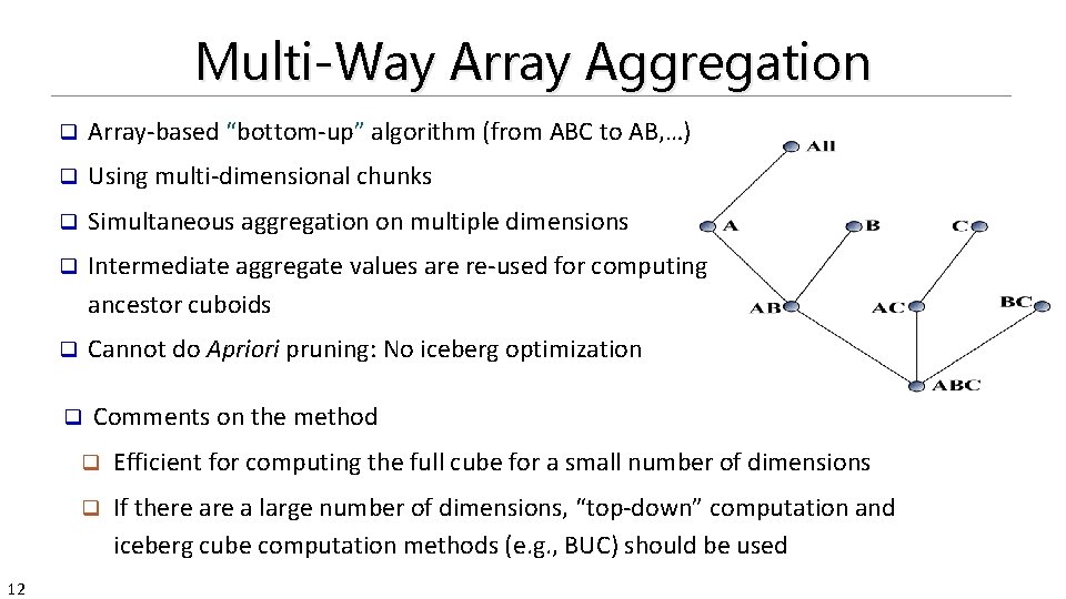
Multi-Way Array Aggregation 12 q Array-based “bottom-up” algorithm (from ABC to AB, …) q Using multi-dimensional chunks q Simultaneous aggregation on multiple dimensions q Intermediate aggregate values are re-used for computing ancestor cuboids q Cannot do Apriori pruning: No iceberg optimization q Comments on the method q Efficient for computing the full cube for a small number of dimensions q If there a large number of dimensions, “top-down” computation and iceberg cube computation methods (e. g. , BUC) should be used

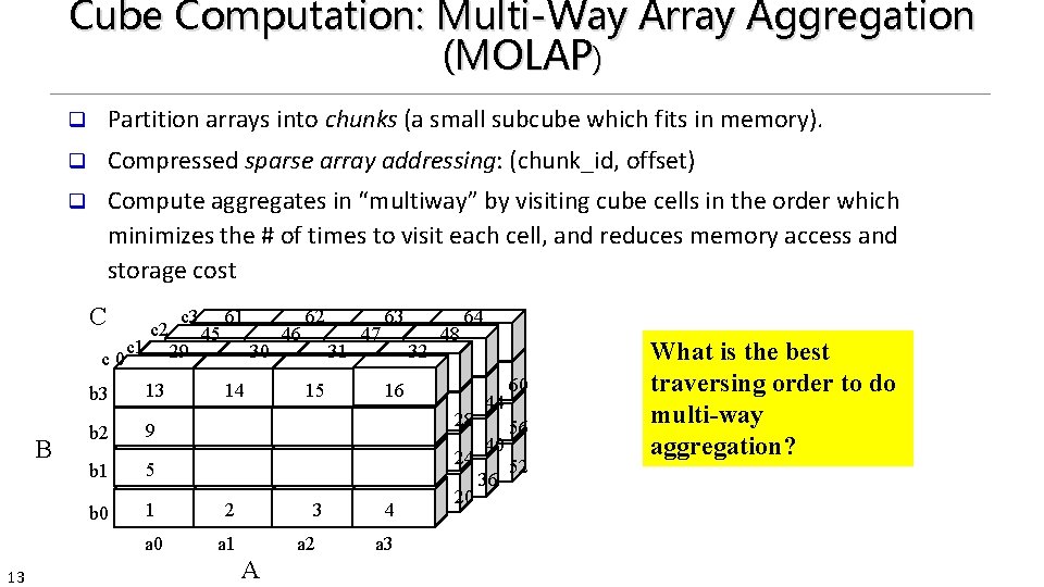
Cube Computation: Multi-Way Array Aggregation (MOLAP) q Partition arrays into chunks (a small subcube which fits in memory). q Compressed sparse array addressing: (chunk_id, offset) q Compute aggregates in “multiway” by visiting cube cells in the order which minimizes the # of times to visit each cell, and reduces memory access and storage cost C c 0 b 3 B 13 b 2 c 1 c 2 B 13 c 3 29 45 61 30 14 46 62 31 15 47 63 32 48 64 16 28 9 24 b 1 5 b 0 1 2 a 0 a 1 3 a 2 A 4 a 3 20 44 40 36 60 56 52 What is the best traversing order to do multi-way aggregation?

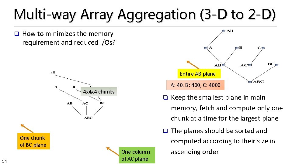
Multi-way Array Aggregation (3 -D to 2 -D) q How to minimizes the memory requirement and reduced I/Os? Entire AB plane A: 40, B: 400, C: 4000 4 x 4 x 4 chunks One chunk of BC plane 14 One column of AC plane q Keep the smallest plane in main memory, fetch and compute only one chunk at a time for the largest plane q The planes should be sorted and computed according to their size in ascending order

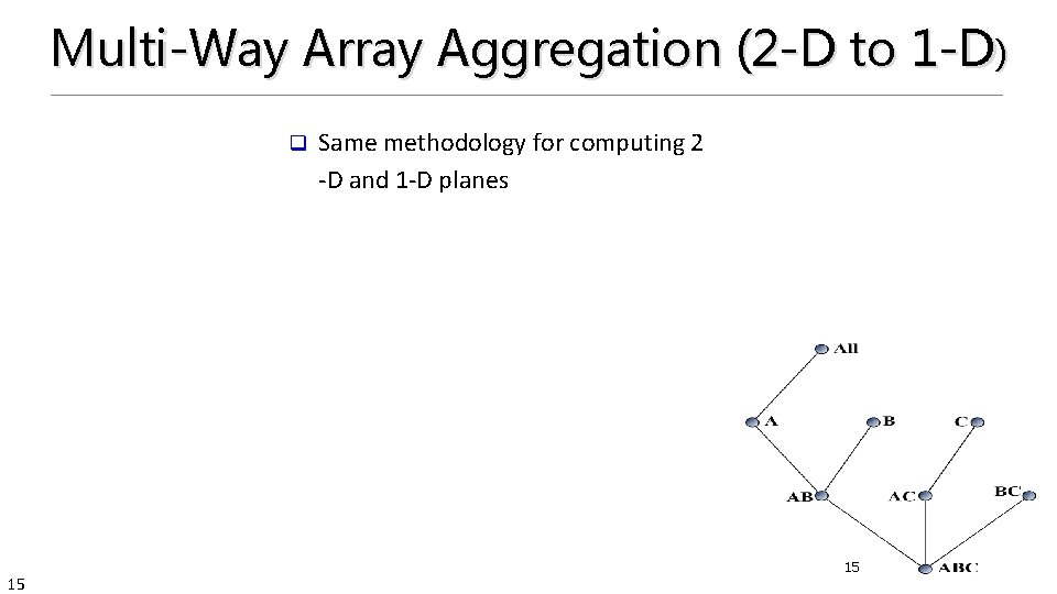
Multi-Way Array Aggregation (2 -D to 1 -D) q 15 Same methodology for computing 2 -D and 1 -D planes 15

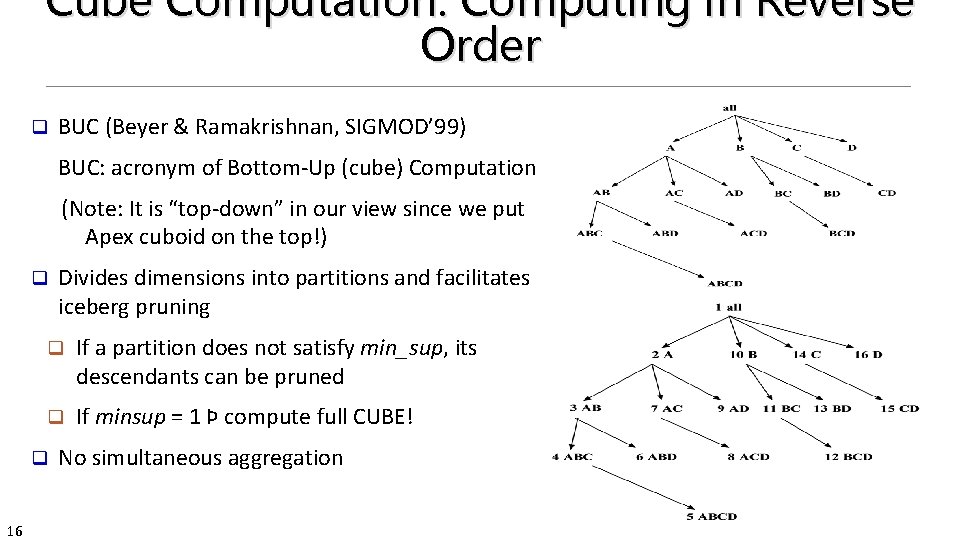
Cube Computation: Computing in Reverse Order q BUC (Beyer & Ramakrishnan, SIGMOD’ 99) BUC: acronym of Bottom-Up (cube) Computation (Note: It is “top-down” in our view since we put Apex cuboid on the top!) q q If a partition does not satisfy min_sup, its descendants can be pruned q If minsup = 1 Þ compute full CUBE! q 16 Divides dimensions into partitions and facilitates iceberg pruning No simultaneous aggregation

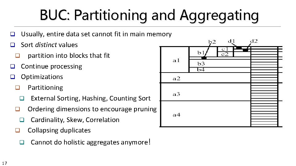
BUC: Partitioning and Aggregating Usually, entire data set cannot fit in main memory q Sort distinct values q partition into blocks that fit q Continue processing q Optimizations q Partitioning q External Sorting, Hashing, Counting Sort q Ordering dimensions to encourage pruning q Cardinality, Skew, Correlation q Collapsing duplicates q q 17 Cannot do holistic aggregates anymore!

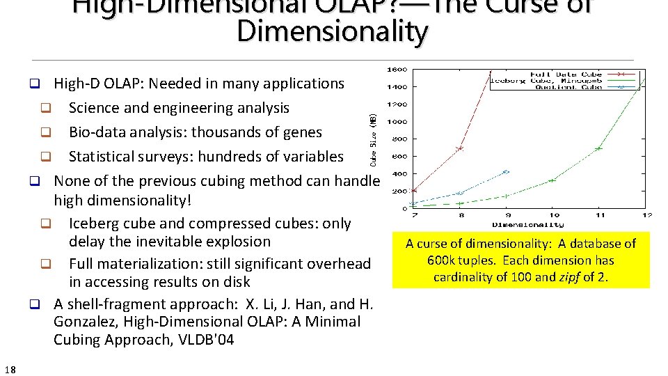
High-Dimensional OLAP? —The Curse of Dimensionality High-D OLAP: Needed in many applications q Science and engineering analysis q Bio-data analysis: thousands of genes q Statistical surveys: hundreds of variables q None of the previous cubing method can handle high dimensionality! q Iceberg cube and compressed cubes: only delay the inevitable explosion q Full materialization: still significant overhead in accessing results on disk q A shell-fragment approach: X. Li, J. Han, and H. Gonzalez, High-Dimensional OLAP: A Minimal Cubing Approach, VLDB'04 q 18 A curse of dimensionality: A database of 600 k tuples. Each dimension has cardinality of 100 and zipf of 2.

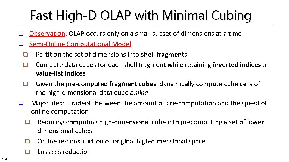
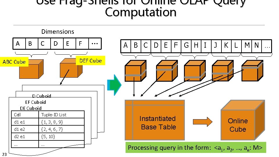
Fast High-D OLAP with Minimal Cubing Observation: OLAP occurs only on a small subset of dimensions at a time q Semi-Online Computational Model q Partition the set of dimensions into shell fragments q Compute data cubes for each shell fragment while retaining inverted indices or value-list indices q Given the pre-computed fragment cubes, dynamically compute cube cells of the high-dimensional data cube online q Major idea: Tradeoff between the amount of pre-computation and the speed of online computation q Reducing computing high-dimensional cube into precomputing a set of lower dimensional cubes q Online re-construction of original high-dimensional space q Lossless reduction q 19

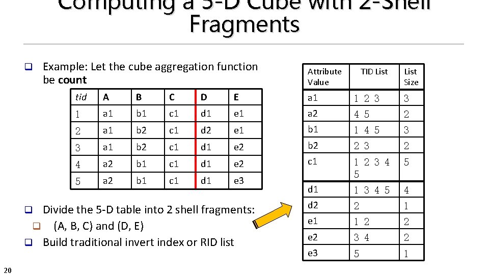
Computing a 5 -D Cube with 2 -Shell Fragments q Example: Let the cube aggregation function be count 20 TID List Size tid A B C D E a 1 1 2 3 3 1 a 1 b 1 c 1 d 1 e 1 a 2 4 5 2 2 a 1 b 2 c 1 d 2 e 1 b 1 1 4 5 3 3 a 1 b 2 c 1 d 1 e 2 b 2 2 3 2 4 a 2 b 1 c 1 d 1 e 2 c 1 5 5 a 2 b 1 c 1 d 1 e 3 1 2 3 4 5 d 1 1 3 4 5 4 d 2 2 1 e 1 1 2 2 e 2 3 4 2 e 3 5 1 Divide the 5 -D table into 2 shell fragments: q (A, B, C) and (D, E) q Build traditional invert index or RID list q Attribute Value

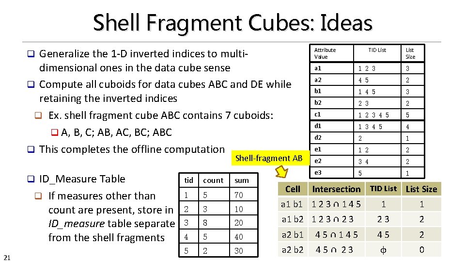
Shell Fragment Cubes: Ideas Generalize the 1 -D inverted indices to multidimensional ones in the data cube sense q Compute all cuboids for data cubes ABC and DE while retaining the inverted indices q Ex. shell fragment cube ABC contains 7 cuboids: q A, B, C; AB, AC, BC; ABC q This completes the offline computation q Shell-fragment AB ID_Measure Table q If measures other than count are present, store in ID_measure table separate from the shell fragments q 21 Attribute Value TID List a 1 1 2 3 3 a 2 4 5 2 b 1 1 4 5 3 b 2 2 3 2 c 1 1 2 3 4 5 5 d 1 1 3 4 5 4 d 2 2 1 e 1 1 2 2 e 2 3 4 2 e 3 5 1 tid count sum 1 5 70 2 3 10 a 1 b 1 1 2 3 ∩ 1 4 5 3 8 20 4 5 5 2 Cell List Size Intersection TID List Size 1 1 a 1 b 2 1 2 3 ∩ 2 3 23 2 40 a 2 b 1 45∩ 145 45 2 30 a 2 b 2 45∩ 23 φ 0

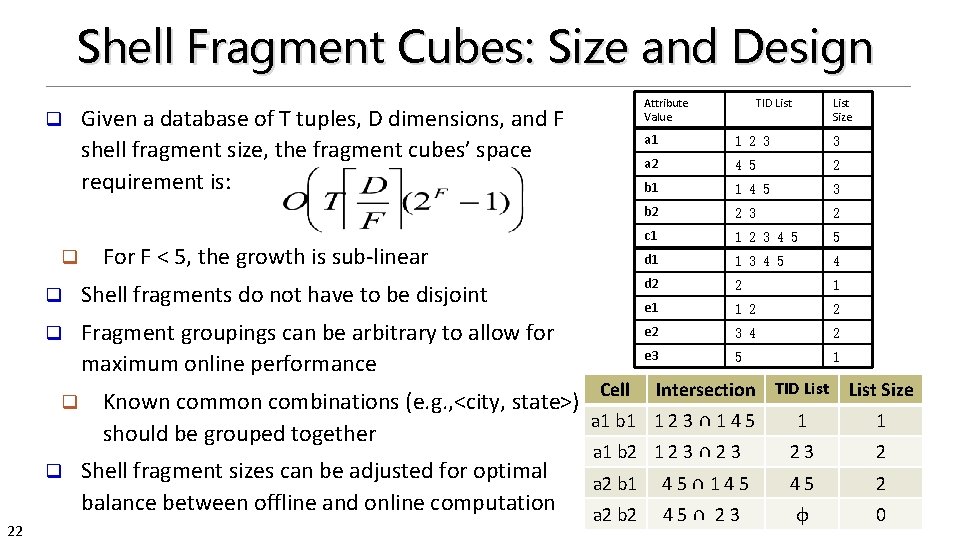
Shell Fragment Cubes: Size and Design q q Given a database of T tuples, D dimensions, and F shell fragment size, the fragment cubes’ space requirement is: For F < 5, the growth is sub-linear TID List Size a 1 1 2 3 3 a 2 4 5 2 b 1 1 4 5 3 b 2 2 3 2 c 1 1 2 3 4 5 5 d 1 1 3 4 5 4 q Shell fragments do not have to be disjoint d 2 2 1 e 1 1 2 2 q Fragment groupings can be arbitrary to allow for maximum online performance e 2 3 4 2 e 3 5 1 q q 22 Attribute Value Cell Intersection TID List Size Known common combinations (e. g. , <city, state>) a 1 b 1 1 2 3 ∩ 1 4 5 should be grouped together Shell fragment sizes can be adjusted for optimal balance between offline and online computation 1 1 a 1 b 2 1 2 3 ∩ 2 3 23 2 a 2 b 1 45∩ 145 45 2 a 2 b 2 45∩ 23 φ 0

Use Frag-Shells for Online OLAP Query Computation Dimensions A B C D E F … A B C D E F G H I J K L M N … DEF Cube ABC Cube D Cuboid EF Cuboid DE Cuboid 23 Cell Tuple-ID List d 1 e 1 {1, 3, 8, 9} d 1 e 2 {2, 4, 6, 7} d 2 e 1 {5, 10} … … Instantiated Base Table Online Cube Processing query in the form: <a 1, a 2, …, an: M>

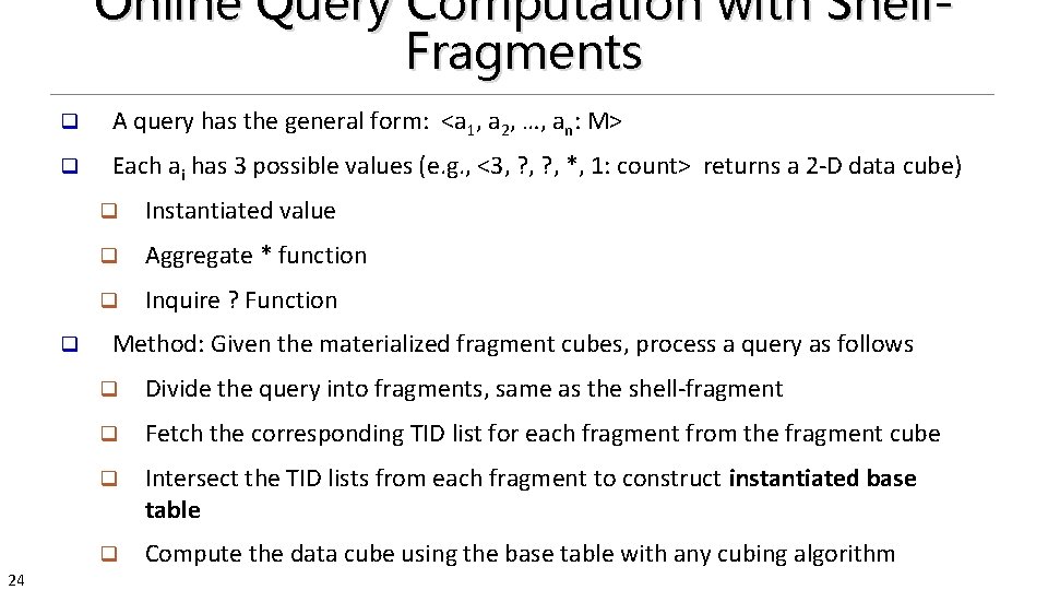
Online Query Computation with Shell. Fragments q A query has the general form: <a 1, a 2, …, an: M> q Each ai has 3 possible values (e. g. , <3, ? , *, 1: count> returns a 2 -D data cube) q 24 q Instantiated value q Aggregate * function q Inquire ? Function Method: Given the materialized fragment cubes, process a query as follows q Divide the query into fragments, same as the shell-fragment q Fetch the corresponding TID list for each fragment from the fragment cube q Intersect the TID lists from each fragment to construct instantiated base table q Compute the data cube using the base table with any cubing algorithm

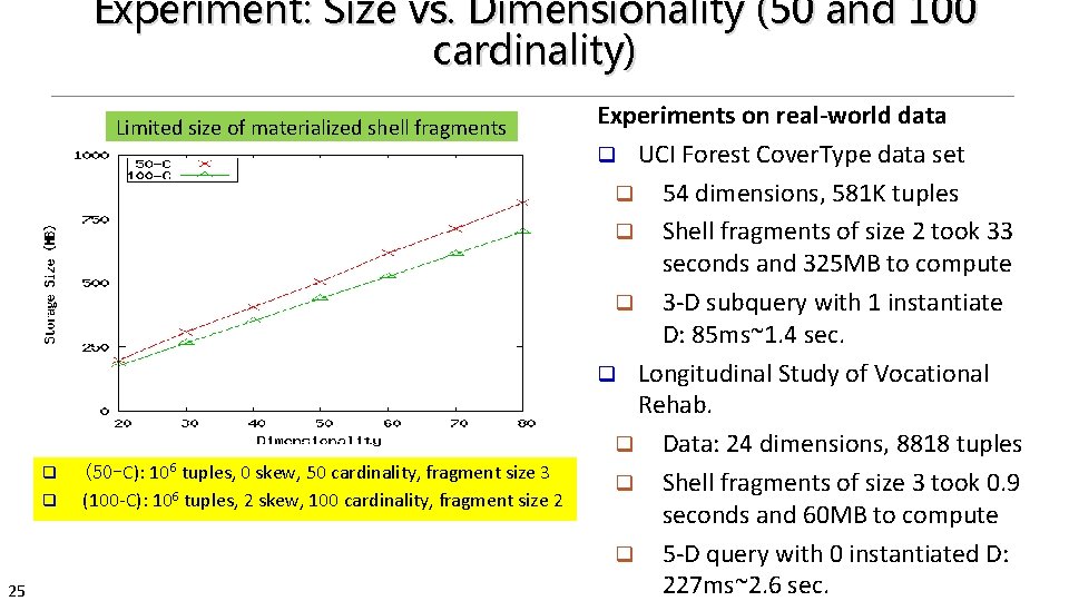
Experiment: Size vs. Dimensionality (50 and 100 cardinality) Limited size of materialized shell fragments q q 25 (50 -C): 106 tuples, 0 skew, 50 cardinality, fragment size 3 (100 -C): 106 tuples, 2 skew, 100 cardinality, fragment size 2 Experiments on real-world data q UCI Forest Cover. Type data set q 54 dimensions, 581 K tuples q Shell fragments of size 2 took 33 seconds and 325 MB to compute q 3 -D subquery with 1 instantiate D: 85 ms~1. 4 sec. q Longitudinal Study of Vocational Rehab. q Data: 24 dimensions, 8818 tuples q Shell fragments of size 3 took 0. 9 seconds and 60 MB to compute q 5 -D query with 0 instantiated D: 227 ms~2. 6 sec.

Chapter 5: Data Cube Technology q Data Cube Computation: Basic Concepts q Data Cube Computation Methods q Processing Advanced Queries with Data Cube Technology q Multidimensional Data Analysis in Cube Space q Summary 26

Chapter 5: Data Cube Technology q Data Cube Computation: Basic Concepts q Data Cube Computation Methods q Processing Advanced Queries with Data Cube Technology q Multidimensional Data Analysis in Cube Space q Summary 27

Data Mining in Cube Space q Data cube greatly increases the analysis bandwidth q Four ways to interact OLAP-styled analysis and data mining q Using cube space to define data space for mining q Using OLAP queries to generate features and targets for mining, e. g. , multi-feature cube q Using data-mining models as building blocks in a multi-step mining process, e. g. , prediction cube q Using data-cube computation techniques to speed up repeated model construction q Cube-space data mining may require building a model for each candidate data space q Sharing computation across model-construction for different candidates may lead 28 to efficient mining

Complex Aggregation at Multiple Granularities: Multi-Feature Cubes Multi-feature cubes (Ross, et al. 1998): Compute complex queries involving multiple dependent aggregates at multiple granularities q Ex. Grouping by all subsets of {item, region, month}, find the maximum price in 2010 for each group, and the total sales among all maximum price tuples select item, region, month, max(price), sum(R. sales) from purchases where year = 2010 cube by item, region, month: R such that R. price = max(price) q Continuing the last example, among the max price tuples, find the min and max shelf live, and find the fraction of the total sales due to tuple that have min shelf life within the set of all max price tuples q 29

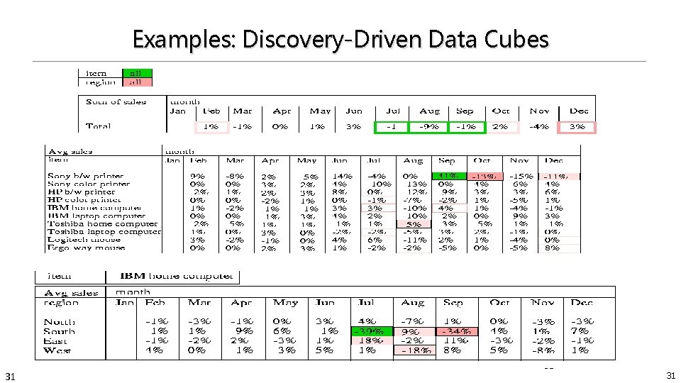
Discovery-Driven Exploration of Data Cubes Discovery-driven exploration of huge cube space (Sarawagi, et al. ’ 98) q Effective navigation of large OLAP data cubes q pre-compute measures indicating exceptions, guide user in the data analysis, at all levels of aggregation q Exception: significantly different from the value anticipated, based on a statistical model q Visual cues such as background color are used to reflect the degree of exception of each cell q Kinds of exceptions q Self. Exp: surprise of cell relative to other cells at same level of aggregation q In. Exp: surprise beneath the cell q Path. Exp: surprise beneath cell for each drill-down path q Computation of exception indicator can be overlapped with cube construction q Exceptions can be stored, indexed and retrieved like precomputed aggregates q 30

Examples: Discovery-Driven Data Cubes 31 31 31

Chapter 5: Data Cube Technology q Data Cube Computation: Basic Concepts q Data Cube Computation Methods q Processing Advanced Queries with Data Cube Technology q Multidimensional Data Analysis in Cube Space q Summary 32

Data Cube Technology: Summary q Data Cube Computation: Preliminary Concepts q Data Cube Computation Methods q Multi. Way Array Aggregation q BUC q High-Dimensional OLAP with Shell-Fragments q 33 Multidimensional Data Analysis in Cube Space q Multi-feature Cubes q Discovery-Driven Exploration of Data Cubes

Data Cube Technology: References (I) q q q q q 34 S. Agarwal, R. Agrawal, P. M. Deshpande, A. Gupta, J. F. Naughton, R. Ramakrishnan, and S. Sarawagi. On the computation of multidimensional aggregates. VLDB’ 96 K. Beyer and R. Ramakrishnan. Bottom-Up Computation of Sparse and Iceberg CUBEs. . SIGMOD’ 99 J. Han, J. Pei, G. Dong, K. Wang. Efficient Computation of Iceberg Cubes With Complex Measures. SIGMOD’ 01 L. V. S. Lakshmanan, J. Pei, and J. Han, Quotient Cube: How to Summarize the Semantics of a Data Cube, VLDB'02 X. Li, J. Han, and H. Gonzalez, High-Dimensional OLAP: A Minimal Cubing Approach, VLDB'04 X. Li, J. Han, Z. Yin, J. -G. Lee, Y. Sun, “Sampling Cube: A Framework for Statistical OLAP over Sampling Data”, SIGMOD’ 08 K. Ross and D. Srivastava. Fast computation of sparse datacubes. VLDB’ 97 D. Xin, J. Han, X. Li, B. W. Wah, Star-Cubing: Computing Iceberg Cubes by Top-Down and Bottom-Up Integration, VLDB'03 Y. Zhao, P. M. Deshpande, and J. F. Naughton. An array-based algorithm for simultaneous multidimensional aggregates. SIGMOD’ 97 D. Burdick, P. Deshpande, T. S. Jayram, R. Ramakrishnan, and S. Vaithyanathan. OLAP over uncertain and imprecise data. VLDB’ 05

Data Cube Technology: References (II) q q q 35 R. Agrawal, A. Gupta, and S. Sarawagi. Modeling multidimensional databases. ICDE’ 97 B. -C. Chen, L. Chen, Y. Lin, and R. Ramakrishnan. Prediction cubes. VLDB’ 05 B. -C. Chen, R. Ramakrishnan, J. W. Shavlik, and P. Tamma. Bellwether analysis: Predicting global aggregates from local regions. VLDB’ 06 Y. Chen, G. Dong, J. Han, B. W. Wah, and J. Wang, Multi-Dimensional Regression Analysis of Time. Series Data Streams, VLDB'02 R. Fagin, R. V. Guha, R. Kumar, J. Novak, D. Sivakumar, and A. Tomkins. Multi-structural databases. PODS’ 05 J. Han. Towards on-line analytical mining in large databases. SIGMOD Record, 27: 97– 107, 1998 T. Imielinski, L. Khachiyan, and A. Abdulghani. Cubegrades: Generalizing association rules. Data Mining & Knowledge Discovery, 6: 219– 258, 2002. R. Ramakrishnan and B. -C. Chen. Exploratory mining in cube space. Data Mining and Knowledge Discovery, 15: 29– 54, 2007. K. A. Ross, D. Srivastava, and D. Chatziantoniou. Complex aggregation at multiple granularities. EDBT'98 S. Sarawagi, R. Agrawal, and N. Megiddo. Discovery-driven exploration of OLAP data cubes. EDBT'98 G. Sathe and S. Sarawagi. Intelligent Rollups in Multidimensional OLAP Data. VLDB'01

36 36