Data Mining Concepts and Techniques Chapter 6 Jiawei

Data Mining: Concepts and Techniques — Chapter 6 — Jiawei Han Department of Computer Science University of Illinois at Urbana-Champaign www. cs. uiuc. edu/~hanj © 2006 Jiawei Han and Micheline Kamber, All rights reserved 12/3/2020 Data Mining: Concepts and Techniques 1

Chapter 6. Classification and Prediction n n What is classification? What is n Support Vector Machines (SVM) prediction? n Associative classification Issues regarding classification n Lazy learners (or learning from and prediction n your neighbors) Classification by decision tree induction n Bayesian classification n Rule-based classification n Classification by back propagation 12/3/2020 n Other classification methods n Prediction n Accuracy and error measures n Ensemble methods n Model selection n Summary Data Mining: Concepts and Techniques 2

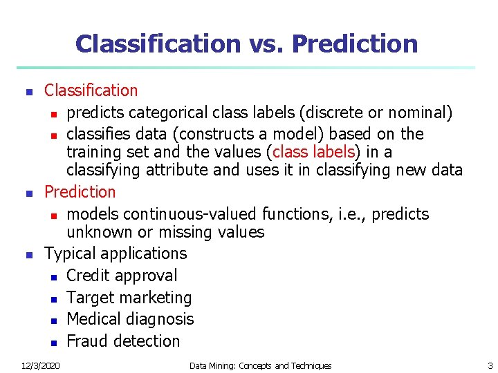
Classification vs. Prediction n Classification n predicts categorical class labels (discrete or nominal) n classifies data (constructs a model) based on the training set and the values (class labels) in a classifying attribute and uses it in classifying new data Prediction n models continuous-valued functions, i. e. , predicts unknown or missing values Typical applications n Credit approval n Target marketing n Medical diagnosis n Fraud detection 12/3/2020 Data Mining: Concepts and Techniques 3

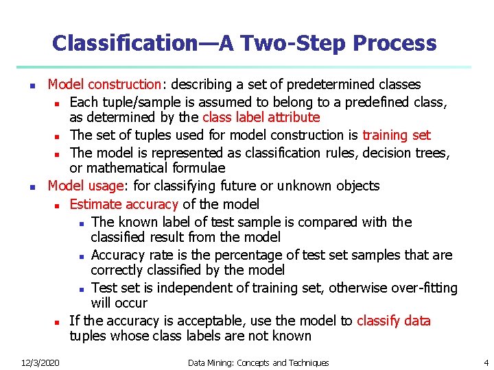
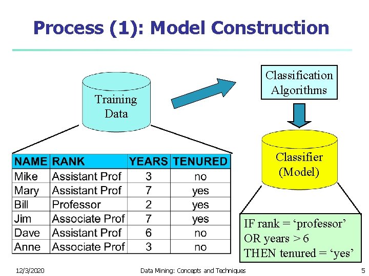
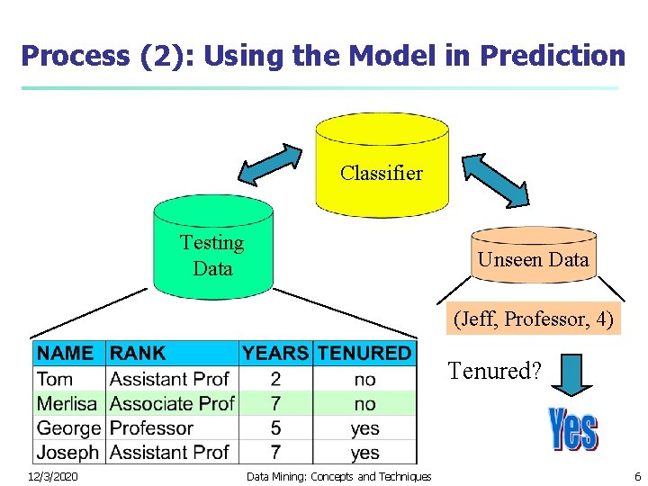
Classification—A Two-Step Process n n Model construction: describing a set of predetermined classes n Each tuple/sample is assumed to belong to a predefined class, as determined by the class label attribute n The set of tuples used for model construction is training set n The model is represented as classification rules, decision trees, or mathematical formulae Model usage: for classifying future or unknown objects n Estimate accuracy of the model n The known label of test sample is compared with the classified result from the model n Accuracy rate is the percentage of test set samples that are correctly classified by the model n Test set is independent of training set, otherwise over-fitting will occur n If the accuracy is acceptable, use the model to classify data tuples whose class labels are not known 12/3/2020 Data Mining: Concepts and Techniques 4

Process (1): Model Construction Classification Algorithms Training Data Classifier (Model) IF rank = ‘professor’ OR years > 6 THEN tenured = ‘yes’ 12/3/2020 Data Mining: Concepts and Techniques 5

Process (2): Using the Model in Prediction Classifier Testing Data Unseen Data (Jeff, Professor, 4) Tenured? 12/3/2020 Data Mining: Concepts and Techniques 6

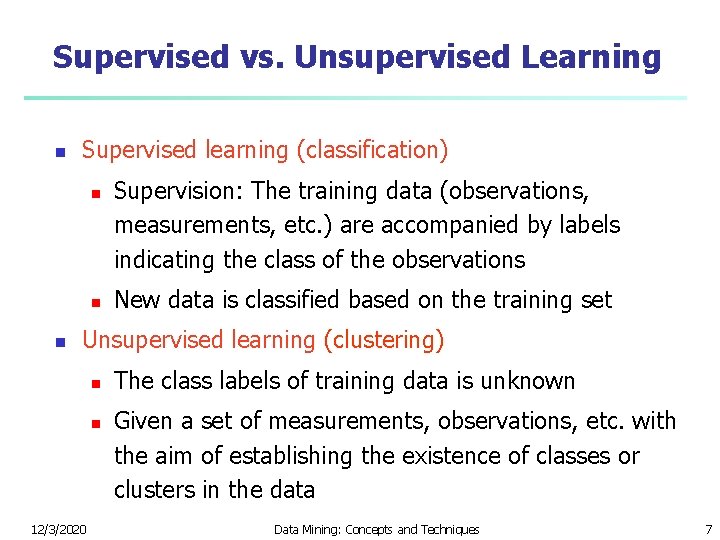
Supervised vs. Unsupervised Learning n Supervised learning (classification) n n n Supervision: The training data (observations, measurements, etc. ) are accompanied by labels indicating the class of the observations New data is classified based on the training set Unsupervised learning (clustering) n n 12/3/2020 The class labels of training data is unknown Given a set of measurements, observations, etc. with the aim of establishing the existence of classes or clusters in the data Data Mining: Concepts and Techniques 7

Chapter 6. Classification and Prediction n n What is classification? What is n Support Vector Machines (SVM) prediction? n Associative classification Issues regarding classification n Lazy learners (or learning from and prediction n your neighbors) Classification by decision tree induction n Bayesian classification n Rule-based classification n Classification by back propagation 12/3/2020 n Other classification methods n Prediction n Accuracy and error measures n Ensemble methods n Model selection n Summary Data Mining: Concepts and Techniques 8

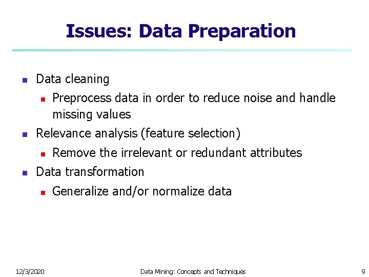
Issues: Data Preparation n Data cleaning n n Relevance analysis (feature selection) n n Preprocess data in order to reduce noise and handle missing values Remove the irrelevant or redundant attributes Data transformation n 12/3/2020 Generalize and/or normalize data Data Mining: Concepts and Techniques 9

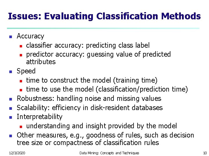
Issues: Evaluating Classification Methods n n n Accuracy n classifier accuracy: predicting class label n predictor accuracy: guessing value of predicted attributes Speed n time to construct the model (training time) n time to use the model (classification/prediction time) Robustness: handling noise and missing values Scalability: efficiency in disk-resident databases Interpretability n understanding and insight provided by the model Other measures, e. g. , goodness of rules, such as decision tree size or compactness of classification rules 12/3/2020 Data Mining: Concepts and Techniques 10

Chapter 6. Classification and Prediction n n What is classification? What is n Support Vector Machines (SVM) prediction? n Associative classification Issues regarding classification n Lazy learners (or learning from and prediction n your neighbors) Classification by decision tree induction n Bayesian classification n Rule-based classification n Classification by back propagation 12/3/2020 n Other classification methods n Prediction n Accuracy and error measures n Ensemble methods n Model selection n Summary Data Mining: Concepts and Techniques 11

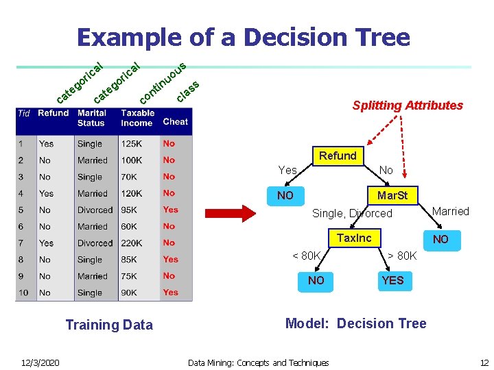
Example of a Decision Tree al ric at c o eg c at al o eg ric in nt co u s u o ss a cl Splitting Attributes Refund Yes No NO Mar. St Single, Divorced Tax. Inc < 80 K NO Training Data 12/3/2020 Married NO > 80 K YES Model: Decision Tree Data Mining: Concepts and Techniques 12

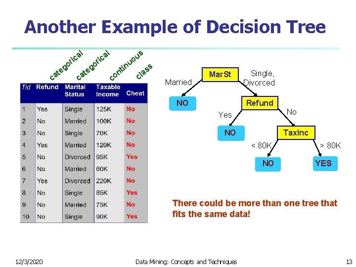
Another Example of Decision Tree l g te ca l a ric o o ca g te s a ric u uo co in t n ss a cl Married Mar. St NO Single, Divorced Refund No Yes NO Tax. Inc < 80 K NO > 80 K YES There could be more than one tree that fits the same data! 12/3/2020 Data Mining: Concepts and Techniques 13

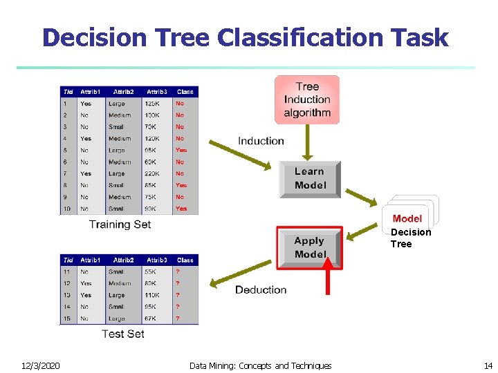
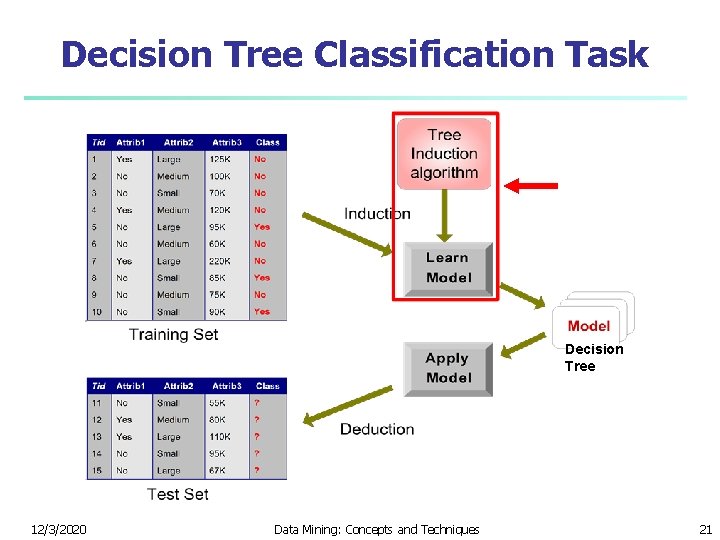
Decision Tree Classification Task Decision Tree 12/3/2020 Data Mining: Concepts and Techniques 14

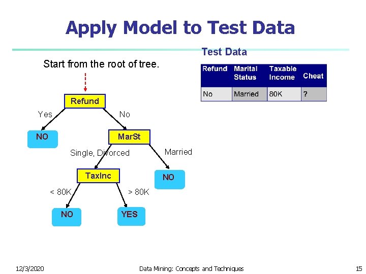
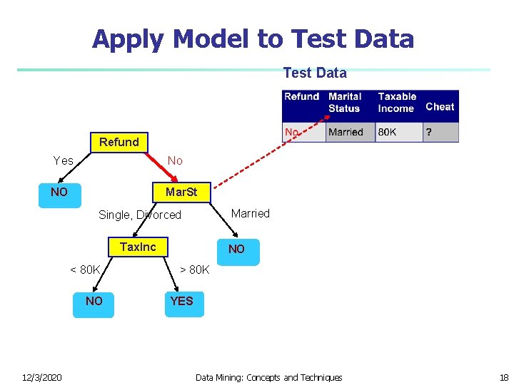
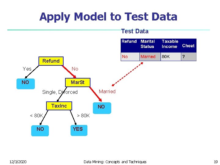
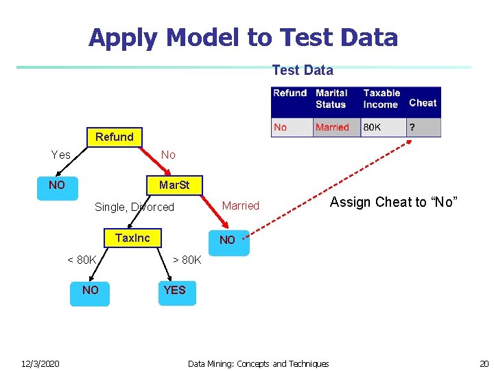
Apply Model to Test Data Start from the root of tree. Refund Yes No NO Mar. St Married Single, Divorced Tax. Inc < 80 K NO 12/3/2020 NO > 80 K YES Data Mining: Concepts and Techniques 15

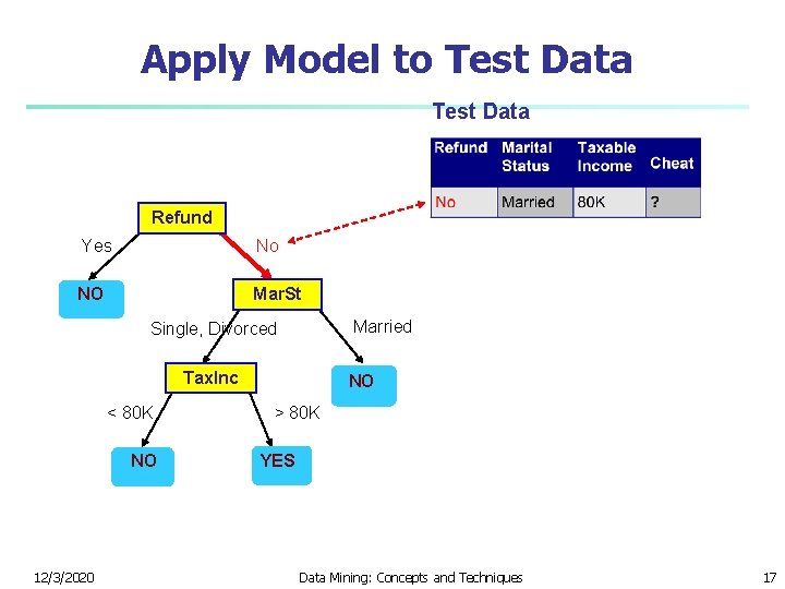
Apply Model to Test Data Refund Yes No NO Mar. St Married Single, Divorced Tax. Inc < 80 K NO 12/3/2020 NO > 80 K YES Data Mining: Concepts and Techniques 16

Apply Model to Test Data Refund Yes No NO Mar. St Married Single, Divorced Tax. Inc < 80 K NO 12/3/2020 NO > 80 K YES Data Mining: Concepts and Techniques 17

Apply Model to Test Data Refund Yes No NO Mar. St Married Single, Divorced Tax. Inc < 80 K NO 12/3/2020 NO > 80 K YES Data Mining: Concepts and Techniques 18

Apply Model to Test Data Refund Yes No NO Mar. St Married Single, Divorced Tax. Inc < 80 K NO 12/3/2020 NO > 80 K YES Data Mining: Concepts and Techniques 19

Apply Model to Test Data Refund Yes No NO Mar. St Married Single, Divorced Tax. Inc < 80 K NO 12/3/2020 Assign Cheat to “No” NO > 80 K YES Data Mining: Concepts and Techniques 20

Decision Tree Classification Task Decision Tree 12/3/2020 Data Mining: Concepts and Techniques 21

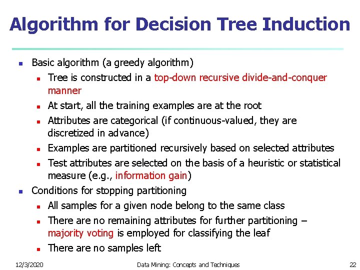
Algorithm for Decision Tree Induction n n Basic algorithm (a greedy algorithm) n Tree is constructed in a top-down recursive divide-and-conquer manner n At start, all the training examples are at the root n Attributes are categorical (if continuous-valued, they are discretized in advance) n Examples are partitioned recursively based on selected attributes n Test attributes are selected on the basis of a heuristic or statistical measure (e. g. , information gain) Conditions for stopping partitioning n All samples for a given node belong to the same class n There are no remaining attributes for further partitioning – majority voting is employed for classifying the leaf n There are no samples left 12/3/2020 Data Mining: Concepts and Techniques 22

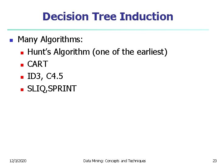
Decision Tree Induction n Many Algorithms: n Hunt’s Algorithm (one of the earliest) n CART n ID 3, C 4. 5 n SLIQ, SPRINT 12/3/2020 Data Mining: Concepts and Techniques 23

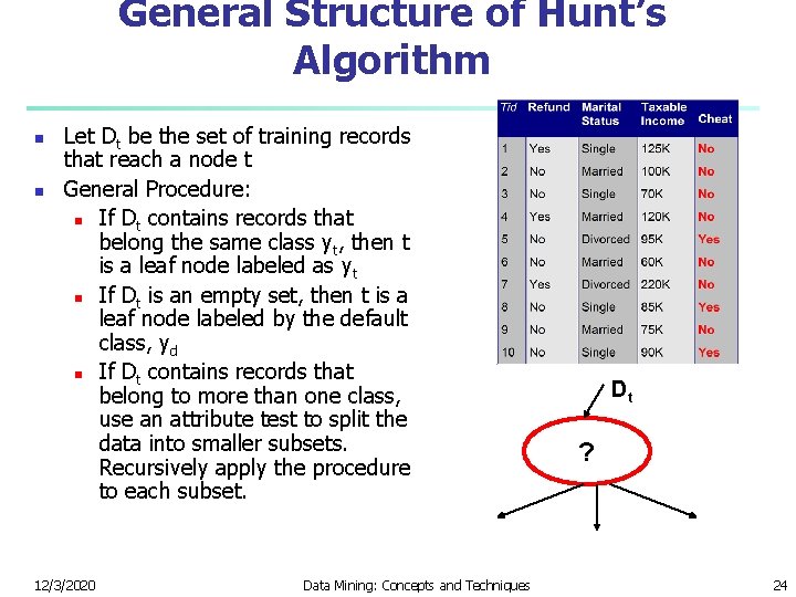
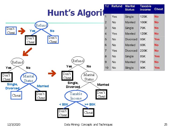
General Structure of Hunt’s Algorithm n n Let Dt be the set of training records that reach a node t General Procedure: n If Dt contains records that belong the same class yt, then t is a leaf node labeled as yt n If Dt is an empty set, then t is a leaf node labeled by the default class, yd n If Dt contains records that belong to more than one class, use an attribute test to split the data into smaller subsets. Recursively apply the procedure to each subset. 12/3/2020 Data Mining: Concepts and Techniques Dt ? 24

Hunt’s Algorithm Don’t Cheat Refund Yes No Don’t Cheat Single, Divorced Cheat 12/3/2020 Don’t Cheat Marital Status Married Single, Divorced No Marital Status Married Don’t Cheat Taxable Income Don’t Cheat < 80 K >= 80 K Don’t Cheat Data Mining: Concepts and Techniques 25

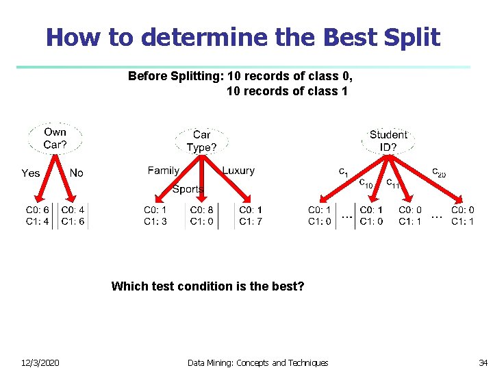
Tree Induction n n Greedy strategy. n Split the records based on an attribute test that optimizes certain criterion. Issues n Determine how to split the records n n n 12/3/2020 How to specify the attribute test condition? How to determine the best split? Determine when to stop splitting Data Mining: Concepts and Techniques 26

Tree Induction n n Greedy strategy. n Split the records based on an attribute test that optimizes certain criterion. Issues n Determine how to split the records n n n 12/3/2020 How to specify the attribute test condition? How to determine the best split? Determine when to stop splitting Data Mining: Concepts and Techniques 27

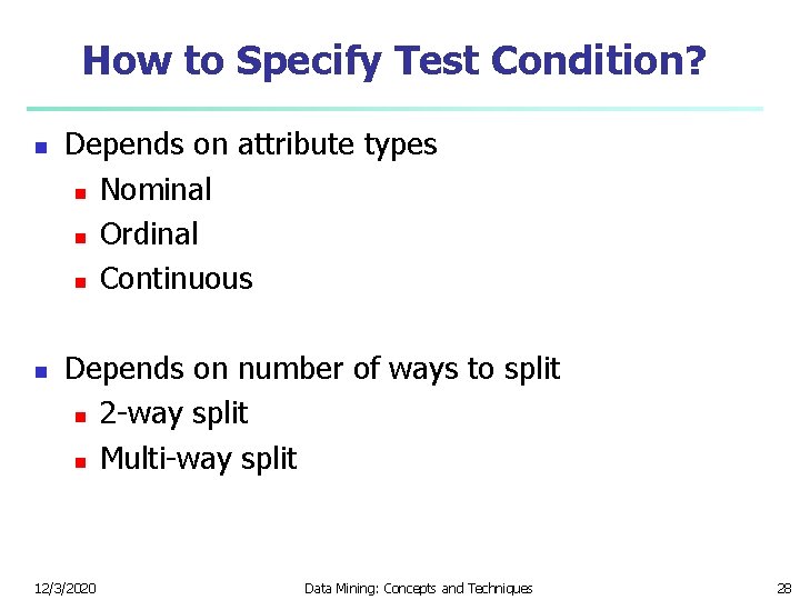
How to Specify Test Condition? n n Depends on attribute types n Nominal n Ordinal n Continuous Depends on number of ways to split n 2 -way split n Multi-way split 12/3/2020 Data Mining: Concepts and Techniques 28

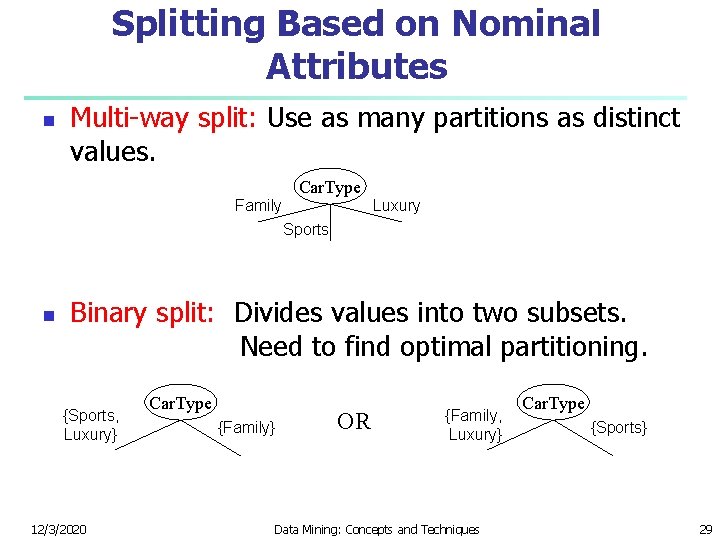
Splitting Based on Nominal Attributes n Multi-way split: Use as many partitions as distinct values. Car. Type Family Luxury Sports n Binary split: Divides values into two subsets. Need to find optimal partitioning. {Sports, Luxury} 12/3/2020 Car. Type {Family} OR {Family, Luxury} Data Mining: Concepts and Techniques Car. Type {Sports} 29

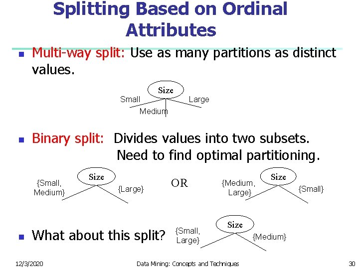
Splitting Based on Ordinal Attributes n Multi-way split: Use as many partitions as distinct values. Size Small Medium n Binary split: Divides values into two subsets. Need to find optimal partitioning. {Small, Medium} n Large Size {Large} What about this split? 12/3/2020 OR {Small, Large} {Medium, Large} Size {Small} Size Data Mining: Concepts and Techniques {Medium} 30

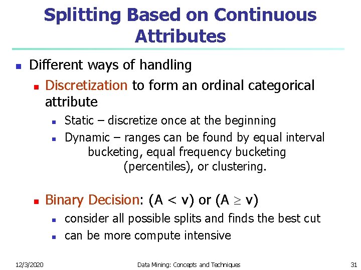
Splitting Based on Continuous Attributes n Different ways of handling n Discretization to form an ordinal categorical attribute n n n Binary Decision: (A < v) or (A v) n n 12/3/2020 Static – discretize once at the beginning Dynamic – ranges can be found by equal interval bucketing, equal frequency bucketing (percentiles), or clustering. consider all possible splits and finds the best cut can be more compute intensive Data Mining: Concepts and Techniques 31

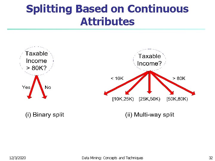
Splitting Based on Continuous Attributes 12/3/2020 Data Mining: Concepts and Techniques 32

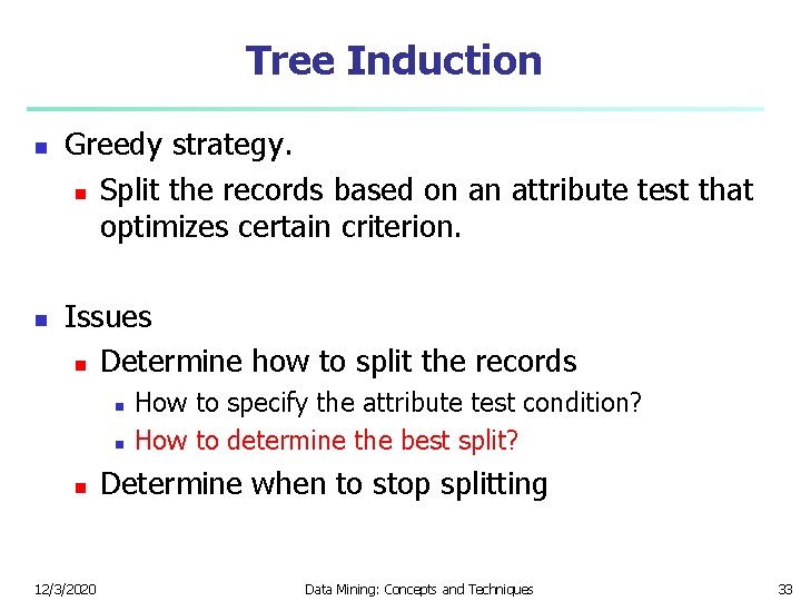
Tree Induction n n Greedy strategy. n Split the records based on an attribute test that optimizes certain criterion. Issues n Determine how to split the records n n n 12/3/2020 How to specify the attribute test condition? How to determine the best split? Determine when to stop splitting Data Mining: Concepts and Techniques 33

How to determine the Best Split Before Splitting: 10 records of class 0, 10 records of class 1 Which test condition is the best? 12/3/2020 Data Mining: Concepts and Techniques 34

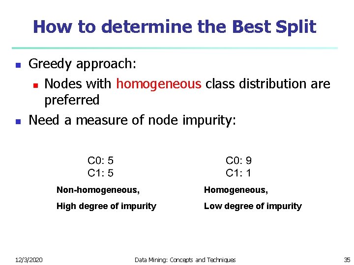
How to determine the Best Split n n Greedy approach: n Nodes with homogeneous class distribution are preferred Need a measure of node impurity: 12/3/2020 Non-homogeneous, High degree of impurity Low degree of impurity Data Mining: Concepts and Techniques 35

Measures of Node Impurity n Gini Index n Entropy n Misclassification error 12/3/2020 Data Mining: Concepts and Techniques 36

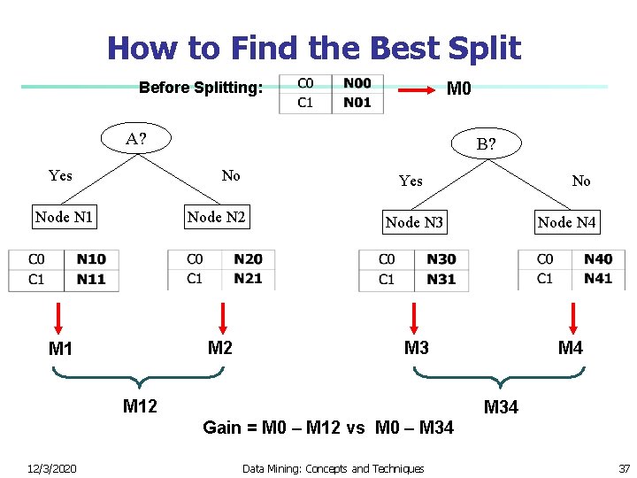
How to Find the Best Split Before Splitting: M 0 A? Yes B? No Yes No Node N 1 Node N 2 Node N 3 Node N 4 M 1 M 2 M 3 M 4 M 12 M 34 Gain = M 0 – M 12 vs M 0 – M 34 12/3/2020 Data Mining: Concepts and Techniques 37

Examples n Using Information Gain 12/3/2020 Data Mining: Concepts and Techniques 38

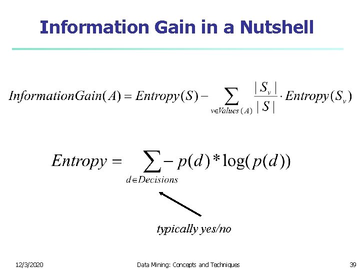
Information Gain in a Nutshell typically yes/no 12/3/2020 Data Mining: Concepts and Techniques 39

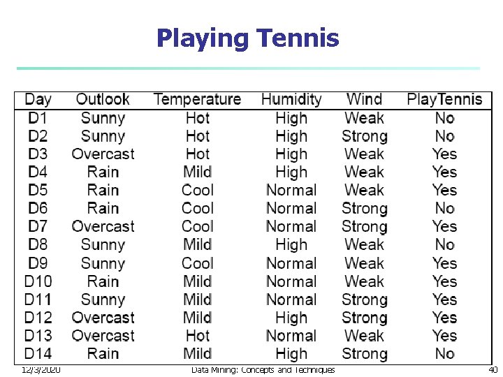
Playing Tennis 12/3/2020 Data Mining: Concepts and Techniques 40

Choosing an Attribute n n We want to split our decision tree on one of the attributes There are four attributes to choose from: n Outlook n Temperature n Humidity n Wind 12/3/2020 Data Mining: Concepts and Techniques 41

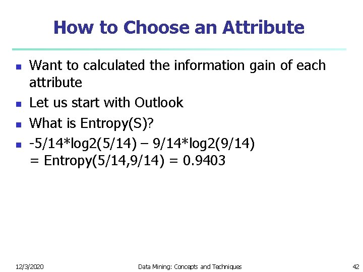
How to Choose an Attribute n n Want to calculated the information gain of each attribute Let us start with Outlook What is Entropy(S)? -5/14*log 2(5/14) – 9/14*log 2(9/14) = Entropy(5/14, 9/14) = 0. 9403 12/3/2020 Data Mining: Concepts and Techniques 42

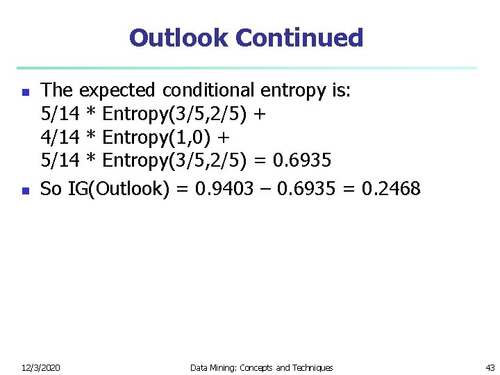
Outlook Continued n n The expected conditional entropy is: 5/14 * Entropy(3/5, 2/5) + 4/14 * Entropy(1, 0) + 5/14 * Entropy(3/5, 2/5) = 0. 6935 So IG(Outlook) = 0. 9403 – 0. 6935 = 0. 2468 12/3/2020 Data Mining: Concepts and Techniques 43

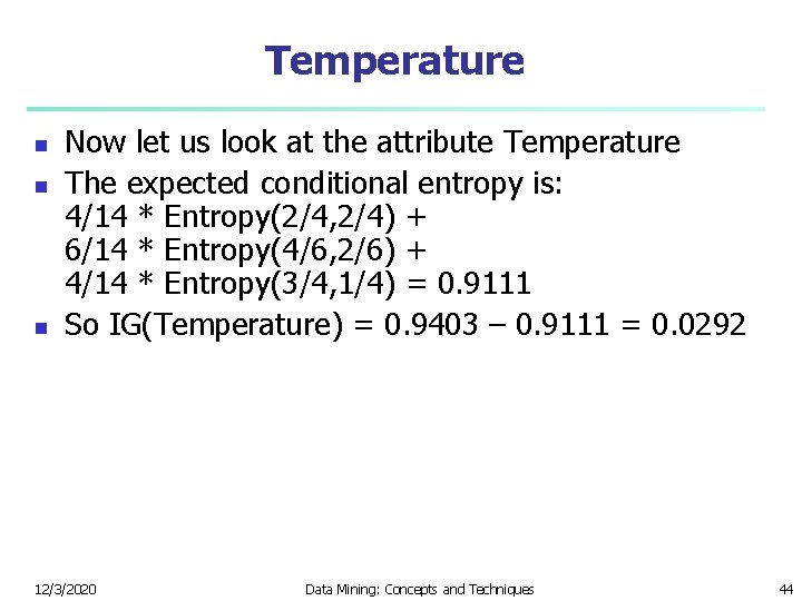
Temperature n n n Now let us look at the attribute Temperature The expected conditional entropy is: 4/14 * Entropy(2/4, 2/4) + 6/14 * Entropy(4/6, 2/6) + 4/14 * Entropy(3/4, 1/4) = 0. 9111 So IG(Temperature) = 0. 9403 – 0. 9111 = 0. 0292 12/3/2020 Data Mining: Concepts and Techniques 44

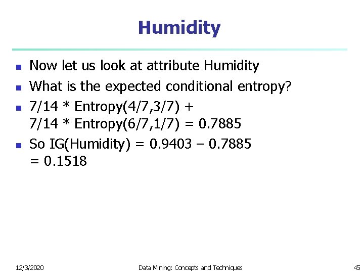
Humidity n n Now let us look at attribute Humidity What is the expected conditional entropy? 7/14 * Entropy(4/7, 3/7) + 7/14 * Entropy(6/7, 1/7) = 0. 7885 So IG(Humidity) = 0. 9403 – 0. 7885 = 0. 1518 12/3/2020 Data Mining: Concepts and Techniques 45

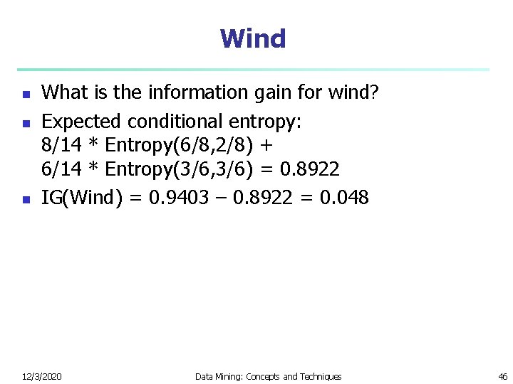
Wind n n n What is the information gain for wind? Expected conditional entropy: 8/14 * Entropy(6/8, 2/8) + 6/14 * Entropy(3/6, 3/6) = 0. 8922 IG(Wind) = 0. 9403 – 0. 8922 = 0. 048 12/3/2020 Data Mining: Concepts and Techniques 46

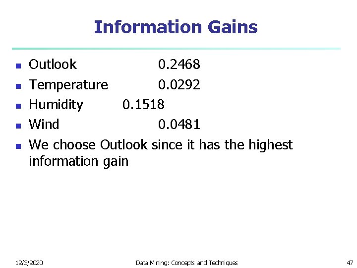
Information Gains n n n Outlook 0. 2468 Temperature 0. 0292 Humidity 0. 1518 Wind 0. 0481 We choose Outlook since it has the highest information gain 12/3/2020 Data Mining: Concepts and Techniques 47

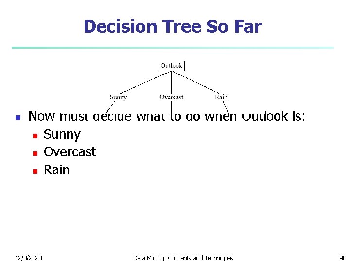
Decision Tree So Far n Now must decide what to do when Outlook is: n Sunny n Overcast n Rain 12/3/2020 Data Mining: Concepts and Techniques 48

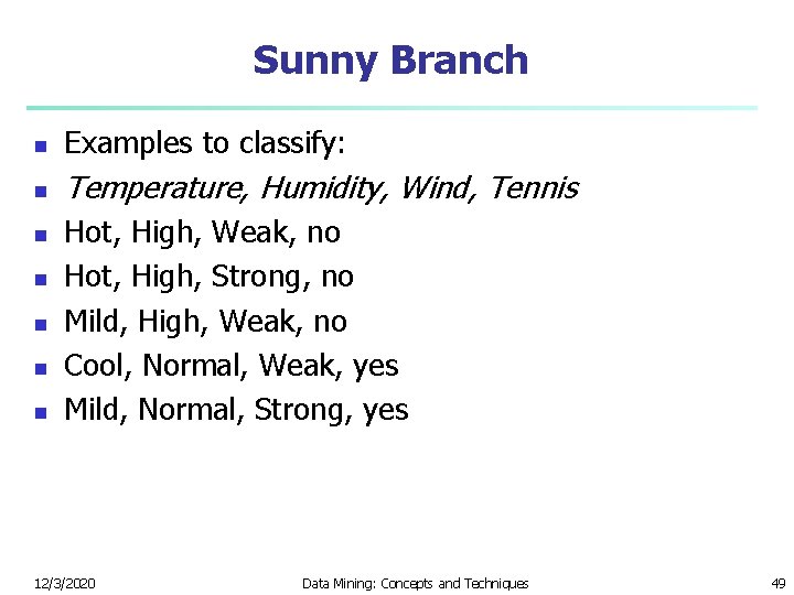
Sunny Branch n Examples to classify: n Temperature, Humidity, Wind, Tennis n n n Hot, High, Weak, no Hot, High, Strong, no Mild, High, Weak, no Cool, Normal, Weak, yes Mild, Normal, Strong, yes 12/3/2020 Data Mining: Concepts and Techniques 49

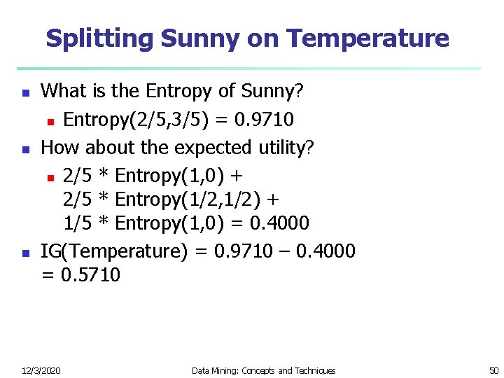
Splitting Sunny on Temperature n n n What is the Entropy of Sunny? n Entropy(2/5, 3/5) = 0. 9710 How about the expected utility? n 2/5 * Entropy(1, 0) + 2/5 * Entropy(1/2, 1/2) + 1/5 * Entropy(1, 0) = 0. 4000 IG(Temperature) = 0. 9710 – 0. 4000 = 0. 5710 12/3/2020 Data Mining: Concepts and Techniques 50

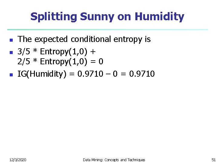
Splitting Sunny on Humidity n n n The expected conditional entropy is 3/5 * Entropy(1, 0) + 2/5 * Entropy(1, 0) = 0 IG(Humidity) = 0. 9710 – 0 = 0. 9710 12/3/2020 Data Mining: Concepts and Techniques 51

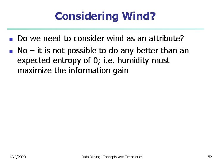
Considering Wind? n n Do we need to consider wind as an attribute? No – it is not possible to do any better than an expected entropy of 0; i. e. humidity must maximize the information gain 12/3/2020 Data Mining: Concepts and Techniques 52

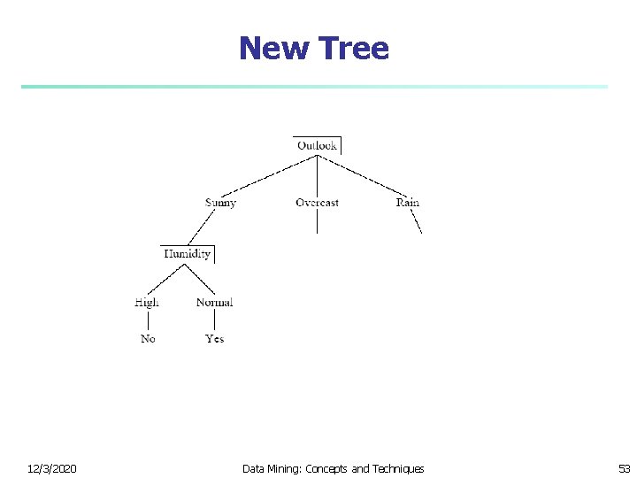
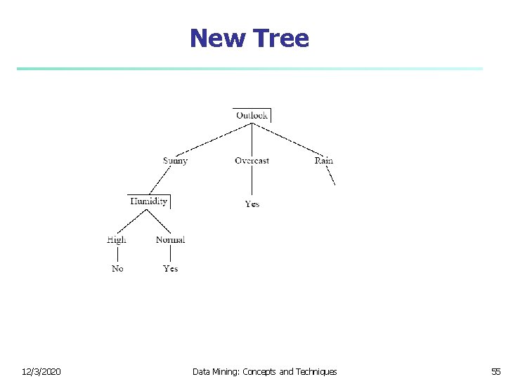
New Tree 12/3/2020 Data Mining: Concepts and Techniques 53

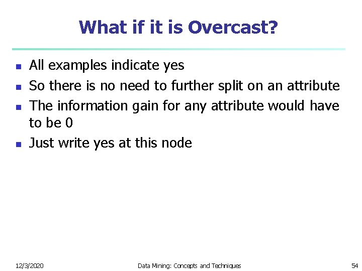
What if it is Overcast? n n All examples indicate yes So there is no need to further split on an attribute The information gain for any attribute would have to be 0 Just write yes at this node 12/3/2020 Data Mining: Concepts and Techniques 54

New Tree 12/3/2020 Data Mining: Concepts and Techniques 55

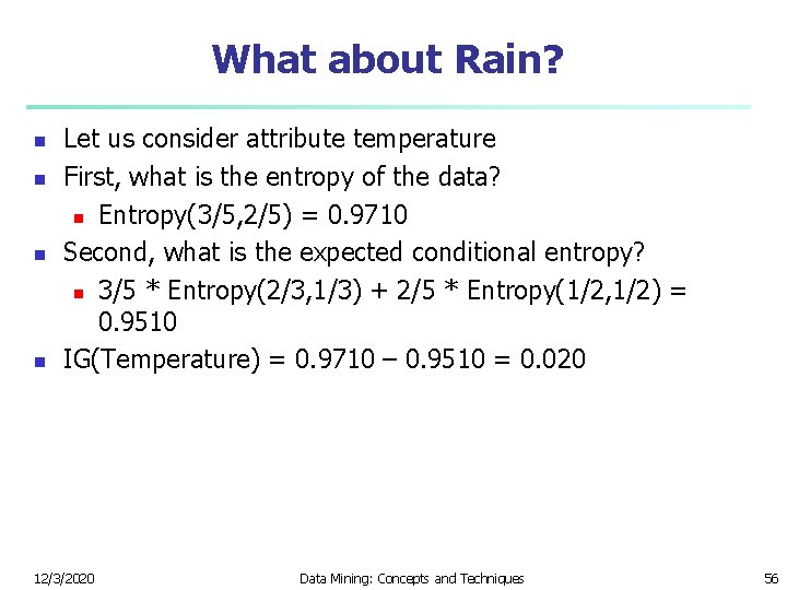
What about Rain? n n Let us consider attribute temperature First, what is the entropy of the data? n Entropy(3/5, 2/5) = 0. 9710 Second, what is the expected conditional entropy? n 3/5 * Entropy(2/3, 1/3) + 2/5 * Entropy(1/2, 1/2) = 0. 9510 IG(Temperature) = 0. 9710 – 0. 9510 = 0. 020 12/3/2020 Data Mining: Concepts and Techniques 56

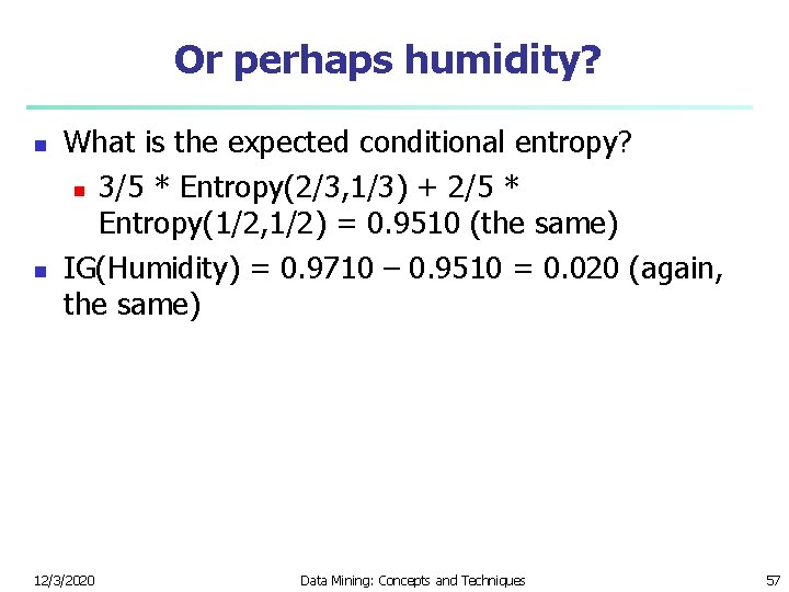
Or perhaps humidity? n n What is the expected conditional entropy? n 3/5 * Entropy(2/3, 1/3) + 2/5 * Entropy(1/2, 1/2) = 0. 9510 (the same) IG(Humidity) = 0. 9710 – 0. 9510 = 0. 020 (again, the same) 12/3/2020 Data Mining: Concepts and Techniques 57

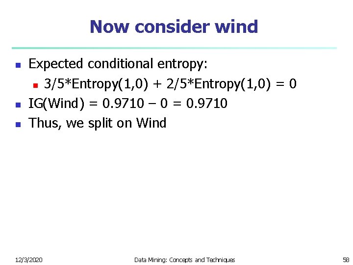
Now consider wind n n n Expected conditional entropy: n 3/5*Entropy(1, 0) + 2/5*Entropy(1, 0) = 0 IG(Wind) = 0. 9710 – 0 = 0. 9710 Thus, we split on Wind 12/3/2020 Data Mining: Concepts and Techniques 58

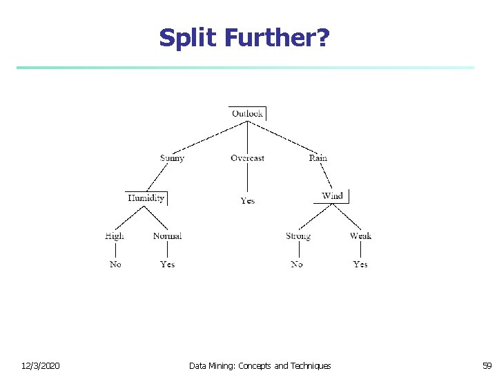
Split Further? 12/3/2020 Data Mining: Concepts and Techniques 59

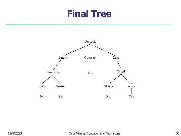
Final Tree 12/3/2020 Data Mining: Concepts and Techniques 60

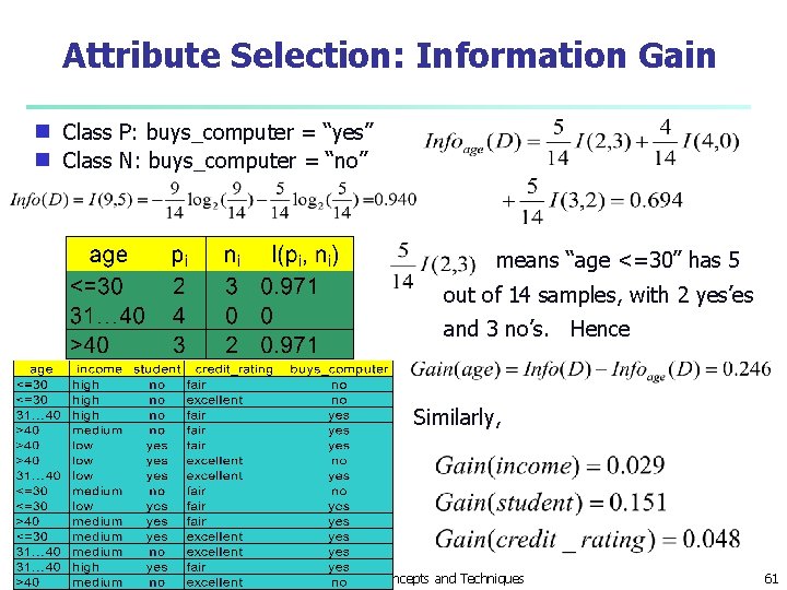
Attribute Selection: Information Gain Class P: buys_computer = “yes” g Class N: buys_computer = “no” g means “age <=30” has 5 out of 14 samples, with 2 yes’es and 3 no’s. Hence Similarly, 12/3/2020 Data Mining: Concepts and Techniques 61

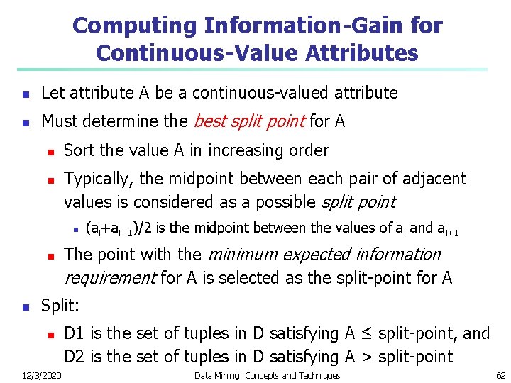
Computing Information-Gain for Continuous-Value Attributes n Let attribute A be a continuous-valued attribute n Must determine the best split point for A n n Sort the value A in increasing order Typically, the midpoint between each pair of adjacent values is considered as a possible split point n n n (ai+ai+1)/2 is the midpoint between the values of ai and ai+1 The point with the minimum expected information requirement for A is selected as the split-point for A Split: n 12/3/2020 D 1 is the set of tuples in D satisfying A ≤ split-point, and D 2 is the set of tuples in D satisfying A > split-point Data Mining: Concepts and Techniques 62

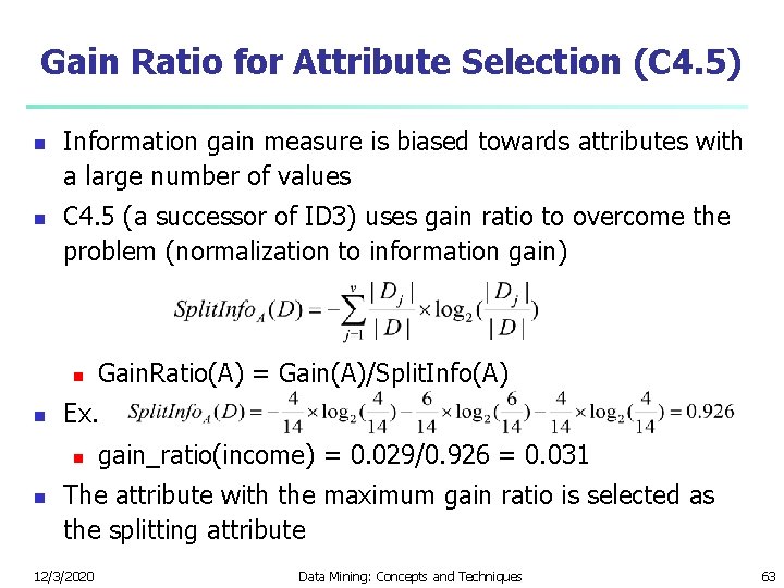
Gain Ratio for Attribute Selection (C 4. 5) n n Information gain measure is biased towards attributes with a large number of values C 4. 5 (a successor of ID 3) uses gain ratio to overcome the problem (normalization to information gain) n n Ex. n n Gain. Ratio(A) = Gain(A)/Split. Info(A) gain_ratio(income) = 0. 029/0. 926 = 0. 031 The attribute with the maximum gain ratio is selected as the splitting attribute 12/3/2020 Data Mining: Concepts and Techniques 63

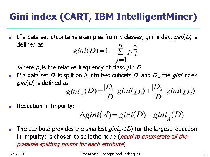
Gini index (CART, IBM Intelligent. Miner) n If a data set D contains examples from n classes, gini index, gini(D) is defined as where pj is the relative frequency of class j in D n If a data set D is split on A into two subsets D 1 and D 2, the gini index gini(D) is defined as n n Reduction in Impurity: The attribute provides the smallest ginisplit(D) (or the largest reduction in impurity) is chosen to split the node (need to enumerate all the possible splitting points for each attribute) 12/3/2020 Data Mining: Concepts and Techniques 64

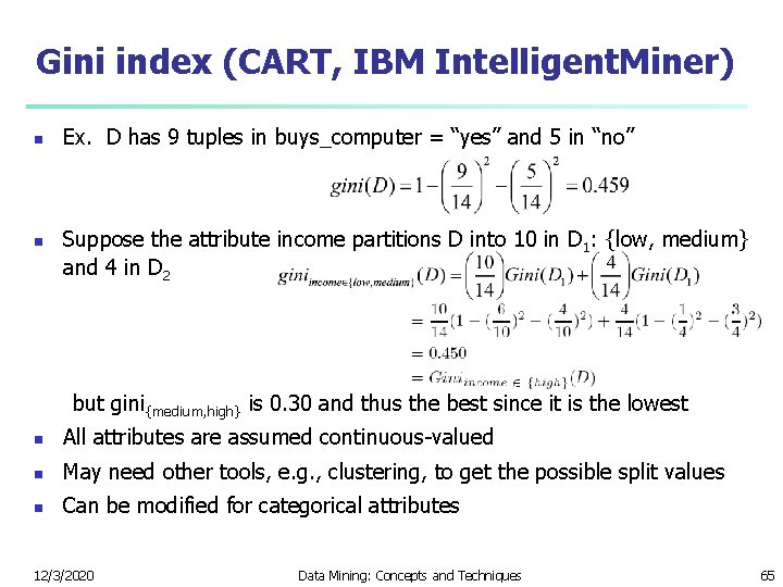
Gini index (CART, IBM Intelligent. Miner) n n Ex. D has 9 tuples in buys_computer = “yes” and 5 in “no” Suppose the attribute income partitions D into 10 in D 1: {low, medium} and 4 in D 2 but gini{medium, high} is 0. 30 and thus the best since it is the lowest n All attributes are assumed continuous-valued n May need other tools, e. g. , clustering, to get the possible split values n Can be modified for categorical attributes 12/3/2020 Data Mining: Concepts and Techniques 65

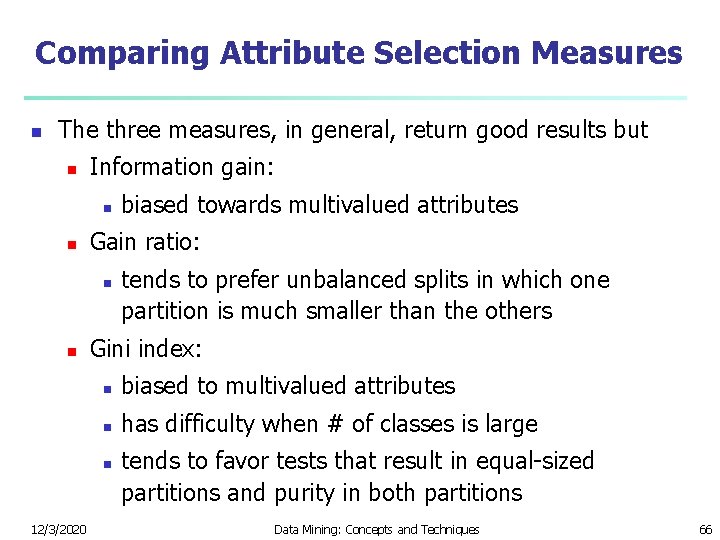
Comparing Attribute Selection Measures n The three measures, in general, return good results but n Information gain: n n Gain ratio: n n tends to prefer unbalanced splits in which one partition is much smaller than the others Gini index: n biased to multivalued attributes n has difficulty when # of classes is large n 12/3/2020 biased towards multivalued attributes tends to favor tests that result in equal-sized partitions and purity in both partitions Data Mining: Concepts and Techniques 66

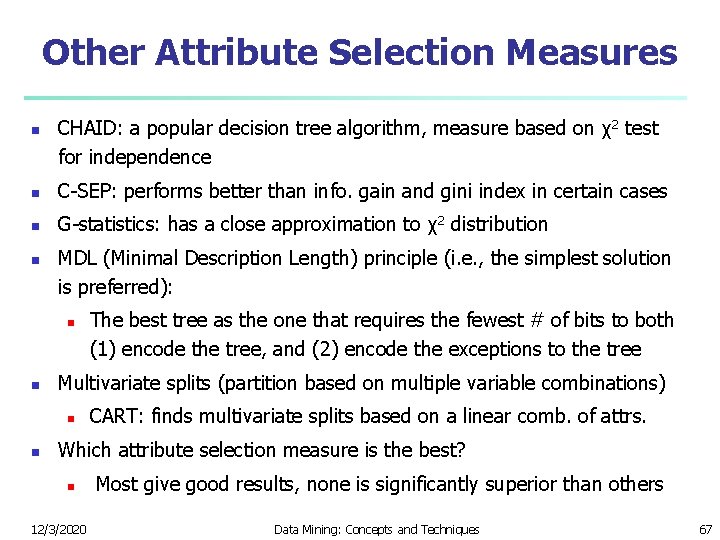
Other Attribute Selection Measures n CHAID: a popular decision tree algorithm, measure based on χ2 test for independence n C-SEP: performs better than info. gain and gini index in certain cases n G-statistics: has a close approximation to χ2 distribution n MDL (Minimal Description Length) principle (i. e. , the simplest solution is preferred): n n Multivariate splits (partition based on multiple variable combinations) n n The best tree as the one that requires the fewest # of bits to both (1) encode the tree, and (2) encode the exceptions to the tree CART: finds multivariate splits based on a linear comb. of attrs. Which attribute selection measure is the best? n 12/3/2020 Most give good results, none is significantly superior than others Data Mining: Concepts and Techniques 67

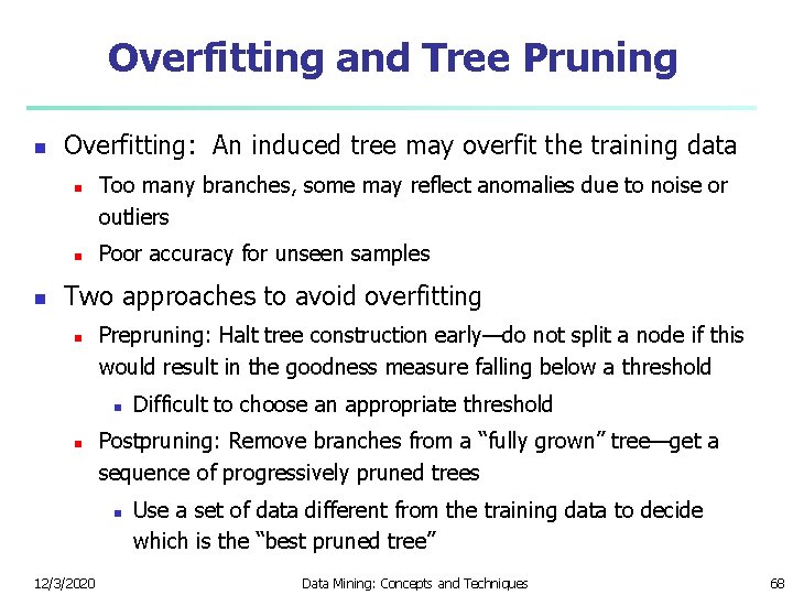
Overfitting and Tree Pruning n Overfitting: An induced tree may overfit the training data n n n Too many branches, some may reflect anomalies due to noise or outliers Poor accuracy for unseen samples Two approaches to avoid overfitting n Prepruning: Halt tree construction early—do not split a node if this would result in the goodness measure falling below a threshold n n Postpruning: Remove branches from a “fully grown” tree—get a sequence of progressively pruned trees n 12/3/2020 Difficult to choose an appropriate threshold Use a set of data different from the training data to decide which is the “best pruned tree” Data Mining: Concepts and Techniques 68

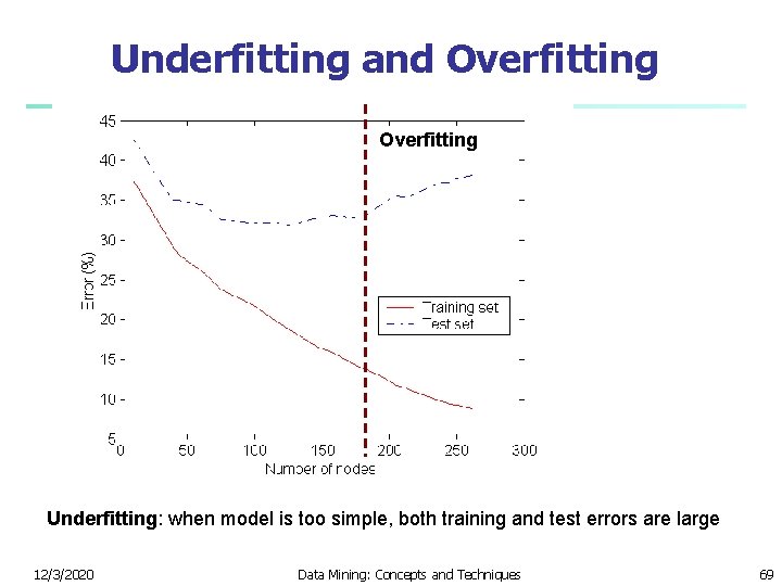
Underfitting and Overfitting Underfitting: when model is too simple, both training and test errors are large 12/3/2020 Data Mining: Concepts and Techniques 69

Overfitting in Classification n Overfitting: An induced tree may overfit the training data n Too many branches, some may reflect anomalies due to noise or outliers n Poor accuracy for unseen samples 12/3/2020 Data Mining: Concepts and Techniques 70

Enhancements to Basic Decision Tree Induction n Allow for continuous-valued attributes n n n Dynamically define new discrete-valued attributes that partition the continuous attribute value into a discrete set of intervals Handle missing attribute values n Assign the most common value of the attribute n Assign probability to each of the possible values Attribute construction n n Create new attributes based on existing ones that are sparsely represented This reduces fragmentation, repetition, and replication 12/3/2020 Data Mining: Concepts and Techniques 71

Classification in Large Databases n n n Classification—a classical problem extensively studied by statisticians and machine learning researchers Scalability: Classifying data sets with millions of examples and hundreds of attributes with reasonable speed Why decision tree induction in data mining? n relatively faster learning speed (than other classification methods) n convertible to simple and easy to understand classification rules n can use SQL queries for accessing databases n comparable classification accuracy with other methods 12/3/2020 Data Mining: Concepts and Techniques 72

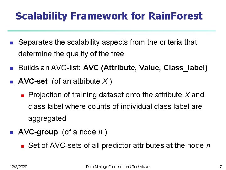
Scalable Decision Tree Induction Methods n n n SLIQ (EDBT’ 96 — Mehta et al. ) n Builds an index for each attribute and only class list and the current attribute list reside in memory SPRINT (VLDB’ 96 — J. Shafer et al. ) n Constructs an attribute list data structure PUBLIC (VLDB’ 98 — Rastogi & Shim) n Integrates tree splitting and tree pruning: stop growing the tree earlier Rain. Forest (VLDB’ 98 — Gehrke, Ramakrishnan & Ganti) n Builds an AVC-list (attribute, value, class label) BOAT (PODS’ 99 — Gehrke, Ganti, Ramakrishnan & Loh) n Uses bootstrapping to create several small samples 12/3/2020 Data Mining: Concepts and Techniques 73

Scalability Framework for Rain. Forest n Separates the scalability aspects from the criteria that determine the quality of the tree n Builds an AVC-list: AVC (Attribute, Value, Class_label) n AVC-set (of an attribute X ) n Projection of training dataset onto the attribute X and class label where counts of individual class label are aggregated n AVC-group (of a node n ) n 12/3/2020 Set of AVC-sets of all predictor attributes at the node n Data Mining: Concepts and Techniques 74

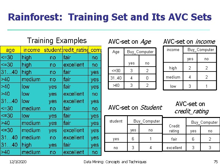
Rainforest: Training Set and Its AVC Sets Training Examples AVC-set on Age Buy_Computer no high 2 2 0 medium 4 2 2 low 3 1 no <=30 3 2 31. . 40 4 >40 3 AVC-set on Student 12/3/2020 income yes student AVC-set on income AVC-set on credit_rating Buy_Computer yes no Credit rating yes 6 1 fair 6 2 no 3 4 excellent 3 3 Data Mining: Concepts and Techniques yes no 75

Chapter 6. Classification and Prediction n n What is classification? What is n Support Vector Machines (SVM) prediction? n Associative classification Issues regarding classification n Lazy learners (or learning from and prediction n your neighbors) Classification by decision tree induction n Bayesian classification n Rule-based classification n Classification by back propagation 12/3/2020 n Other classification methods n Prediction n Accuracy and error measures n Ensemble methods n Model selection n Summary Data Mining: Concepts and Techniques 76

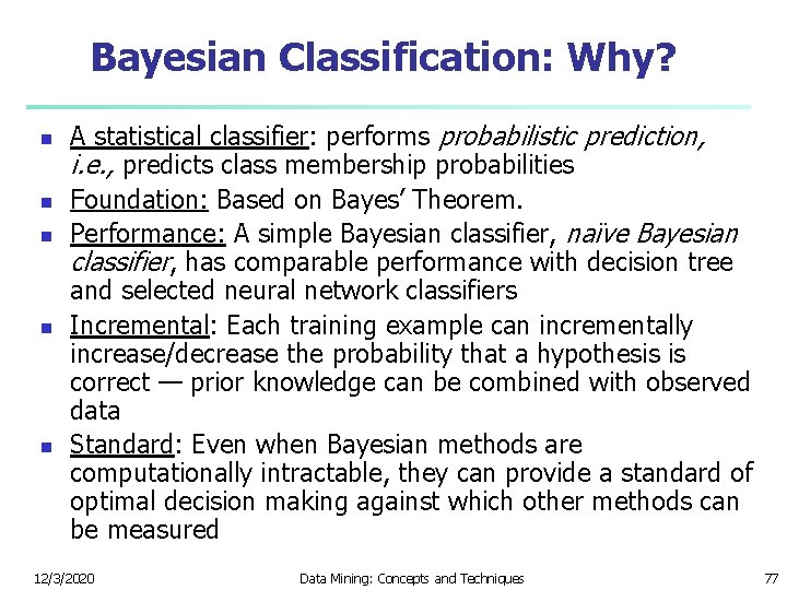
Bayesian Classification: Why? n n n A statistical classifier: performs probabilistic prediction, i. e. , predicts class membership probabilities Foundation: Based on Bayes’ Theorem. Performance: A simple Bayesian classifier, naïve Bayesian classifier, has comparable performance with decision tree and selected neural network classifiers Incremental: Each training example can incrementally increase/decrease the probability that a hypothesis is correct — prior knowledge can be combined with observed data Standard: Even when Bayesian methods are computationally intractable, they can provide a standard of optimal decision making against which other methods can be measured 12/3/2020 Data Mining: Concepts and Techniques 77

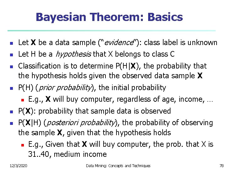
Bayesian Theorem: Basics n Let X be a data sample (“evidence”): class label is unknown n Let H be a hypothesis that X belongs to class C n n Classification is to determine P(H|X), the probability that the hypothesis holds given the observed data sample X P(H) (prior probability), the initial probability n n n E. g. , X will buy computer, regardless of age, income, … P(X): probability that sample data is observed P(X|H) (posteriori probability), the probability of observing the sample X, given that the hypothesis holds n 12/3/2020 E. g. , Given that X will buy computer, the prob. that X is 31. . 40, medium income Data Mining: Concepts and Techniques 78

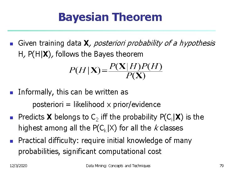
Bayesian Theorem n n Given training data X, posteriori probability of a hypothesis H, P(H|X), follows the Bayes theorem Informally, this can be written as posteriori = likelihood x prior/evidence n n Predicts X belongs to C 2 iff the probability P(Ci|X) is the highest among all the P(Ck|X) for all the k classes Practical difficulty: require initial knowledge of many probabilities, significant computational cost 12/3/2020 Data Mining: Concepts and Techniques 79

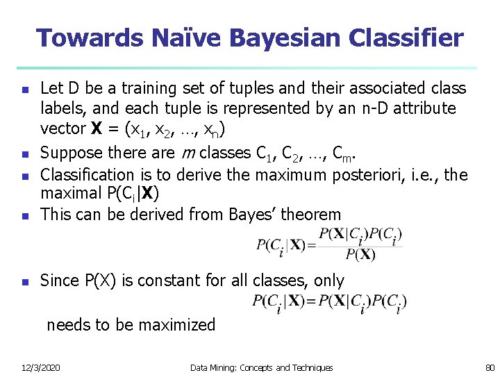
Towards Naïve Bayesian Classifier n Let D be a training set of tuples and their associated class labels, and each tuple is represented by an n-D attribute vector X = (x 1, x 2, …, xn) Suppose there are m classes C 1, C 2, …, Cm. Classification is to derive the maximum posteriori, i. e. , the maximal P(Ci|X) This can be derived from Bayes’ theorem n Since P(X) is constant for all classes, only n needs to be maximized 12/3/2020 Data Mining: Concepts and Techniques 80

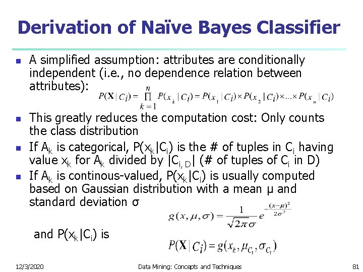
Derivation of Naïve Bayes Classifier n n A simplified assumption: attributes are conditionally independent (i. e. , no dependence relation between attributes): This greatly reduces the computation cost: Only counts the class distribution If Ak is categorical, P(xk|Ci) is the # of tuples in Ci having value xk for Ak divided by |Ci, D| (# of tuples of Ci in D) If Ak is continous-valued, P(xk|Ci) is usually computed based on Gaussian distribution with a mean μ and standard deviation σ and P(xk|Ci) is 12/3/2020 Data Mining: Concepts and Techniques 81

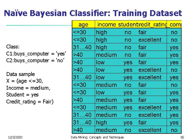
Naïve Bayesian Classifier: Training Dataset Class: C 1: buys_computer = ‘yes’ C 2: buys_computer = ‘no’ Data sample X = (age <=30, Income = medium, Student = yes Credit_rating = Fair) 12/3/2020 Data Mining: Concepts and Techniques 82

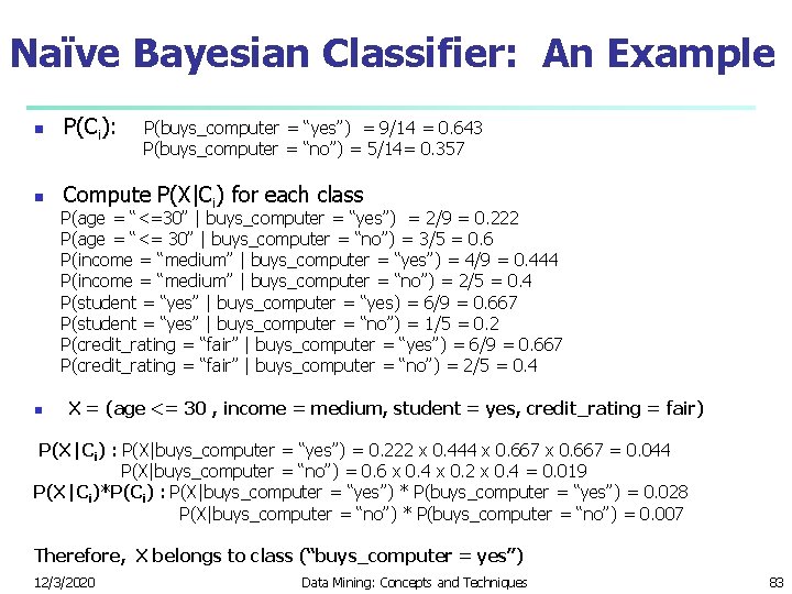
Naïve Bayesian Classifier: An Example n P(Ci): P(buys_computer = “yes”) = 9/14 = 0. 643 P(buys_computer = “no”) = 5/14= 0. 357 n Compute P(X|Ci) for each class P(age = “<=30” | buys_computer = “yes”) = 2/9 = 0. 222 P(age = “<= 30” | buys_computer = “no”) = 3/5 = 0. 6 P(income = “medium” | buys_computer = “yes”) = 4/9 = 0. 444 P(income = “medium” | buys_computer = “no”) = 2/5 = 0. 4 P(student = “yes” | buys_computer = “yes) = 6/9 = 0. 667 P(student = “yes” | buys_computer = “no”) = 1/5 = 0. 2 P(credit_rating = “fair” | buys_computer = “yes”) = 6/9 = 0. 667 P(credit_rating = “fair” | buys_computer = “no”) = 2/5 = 0. 4 n X = (age <= 30 , income = medium, student = yes, credit_rating = fair) P(X|Ci) : P(X|buys_computer = “yes”) = 0. 222 x 0. 444 x 0. 667 = 0. 044 P(X|buys_computer = “no”) = 0. 6 x 0. 4 x 0. 2 x 0. 4 = 0. 019 P(X|Ci)*P(Ci) : P(X|buys_computer = “yes”) * P(buys_computer = “yes”) = 0. 028 P(X|buys_computer = “no”) * P(buys_computer = “no”) = 0. 007 Therefore, X belongs to class (“buys_computer = yes”) 12/3/2020 Data Mining: Concepts and Techniques 83

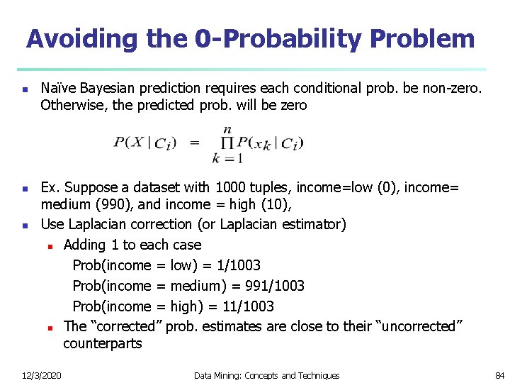
Avoiding the 0 -Probability Problem n n n Naïve Bayesian prediction requires each conditional prob. be non-zero. Otherwise, the predicted prob. will be zero Ex. Suppose a dataset with 1000 tuples, income=low (0), income= medium (990), and income = high (10), Use Laplacian correction (or Laplacian estimator) n Adding 1 to each case Prob(income = low) = 1/1003 Prob(income = medium) = 991/1003 Prob(income = high) = 11/1003 n The “corrected” prob. estimates are close to their “uncorrected” counterparts 12/3/2020 Data Mining: Concepts and Techniques 84

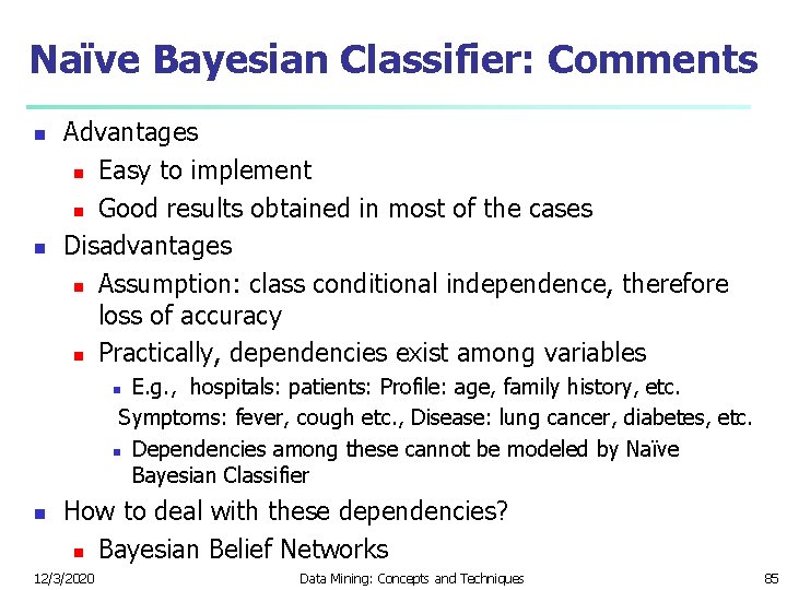
Naïve Bayesian Classifier: Comments n n Advantages n Easy to implement n Good results obtained in most of the cases Disadvantages n Assumption: class conditional independence, therefore loss of accuracy n Practically, dependencies exist among variables E. g. , hospitals: patients: Profile: age, family history, etc. Symptoms: fever, cough etc. , Disease: lung cancer, diabetes, etc. n Dependencies among these cannot be modeled by Naïve Bayesian Classifier n n How to deal with these dependencies? n Bayesian Belief Networks 12/3/2020 Data Mining: Concepts and Techniques 85

Chapter 6. Classification and Prediction n n What is classification? What is n Support Vector Machines (SVM) prediction? n Associative classification Issues regarding classification n Lazy learners (or learning from and prediction n your neighbors) Classification by decision tree induction n Bayesian classification n Rule-based classification n Classification by back propagation 12/3/2020 n Other classification methods n Prediction n Accuracy and error measures n Ensemble methods n Model selection n Summary Data Mining: Concepts and Techniques 86

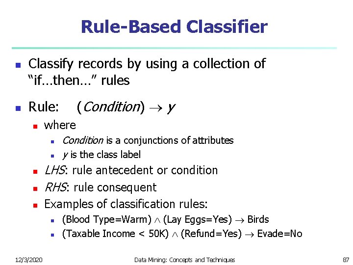
Rule-Based Classifier n n Classify records by using a collection of “if…then…” rules Rule: (Condition) y n where n n Condition is a conjunctions of attributes y is the class label n LHS: rule antecedent or condition RHS: rule consequent n Examples of classification rules: n n n 12/3/2020 (Blood Type=Warm) (Lay Eggs=Yes) Birds (Taxable Income < 50 K) (Refund=Yes) Evade=No Data Mining: Concepts and Techniques 87

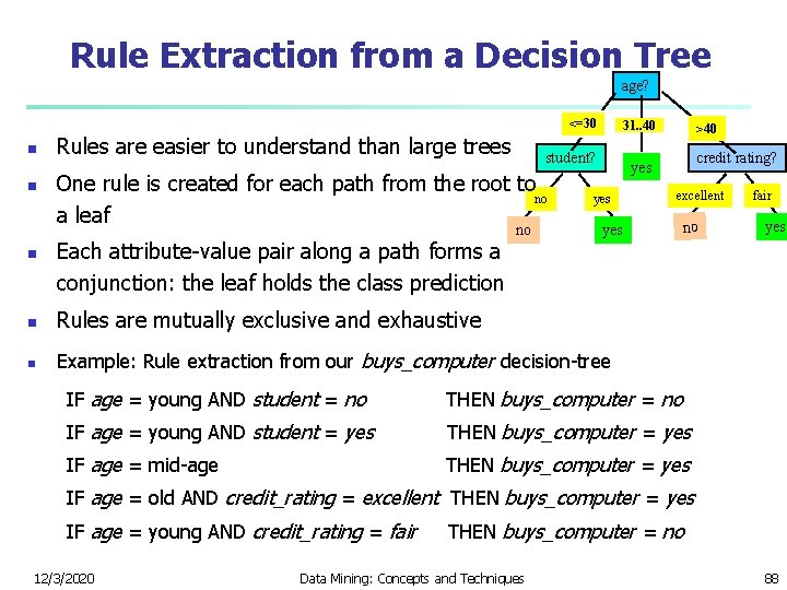
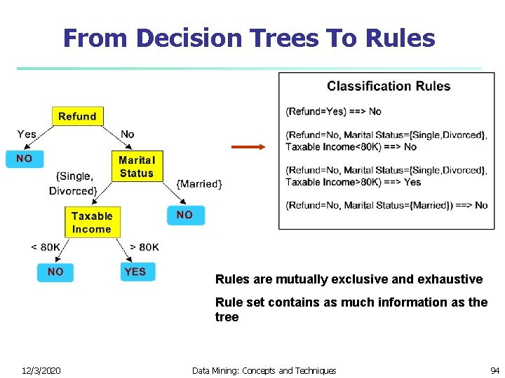
Rule Extraction from a Decision Tree age? <=30 n n n Rules are easier to understand than large trees student? One rule is created for each path from the root to no a leaf Each attribute-value pair along a path forms a conjunction: the leaf holds the class prediction 31. . 40 no >40 credit rating? yes yes n Rules are mutually exclusive and exhaustive n Example: Rule extraction from our buys_computer decision-tree excellent no fair yes IF age = young AND student = no THEN buys_computer = no IF age = young AND student = yes THEN buys_computer = yes IF age = mid-age THEN buys_computer = yes IF age = old AND credit_rating = excellent THEN buys_computer = yes IF age = young AND credit_rating = fair THEN buys_computer = no 12/3/2020 Data Mining: Concepts and Techniques 88

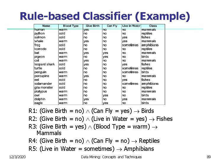
Rule-based Classifier (Example) R 1: (Give Birth = no) (Can Fly = yes) Birds R 2: (Give Birth = no) (Live in Water = yes) Fishes R 3: (Give Birth = yes) (Blood Type = warm) Mammals R 4: (Give Birth = no) (Can Fly = no) Reptiles R 5: (Live in Water = sometimes) Amphibians 12/3/2020 Data Mining: Concepts and Techniques 89

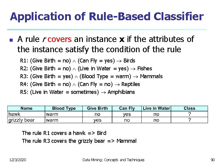
Application of Rule-Based Classifier n A rule r covers an instance x if the attributes of the instance satisfy the condition of the rule R 1: (Give Birth = no) (Can Fly = yes) Birds R 2: (Give Birth = no) (Live in Water = yes) Fishes R 3: (Give Birth = yes) (Blood Type = warm) Mammals R 4: (Give Birth = no) (Can Fly = no) Reptiles R 5: (Live in Water = sometimes) Amphibians The rule R 1 covers a hawk => Bird The rule R 3 covers the grizzly bear => Mammal 12/3/2020 Data Mining: Concepts and Techniques 90

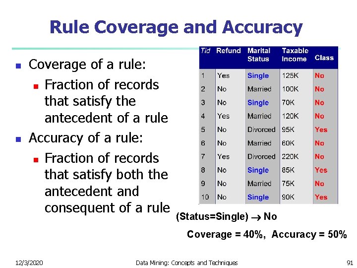
Rule Coverage and Accuracy n n Coverage of a rule: n Fraction of records that satisfy the antecedent of a rule Accuracy of a rule: n Fraction of records that satisfy both the antecedent and consequent of a rule (Status=Single) No Coverage = 40%, Accuracy = 50% 12/3/2020 Data Mining: Concepts and Techniques 91

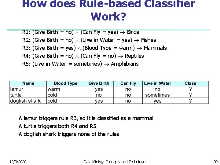
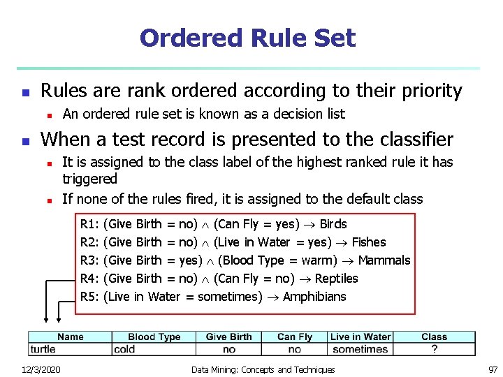
How does Rule-based Classifier Work? R 1: (Give Birth = no) (Can Fly = yes) Birds R 2: (Give Birth = no) (Live in Water = yes) Fishes R 3: (Give Birth = yes) (Blood Type = warm) Mammals R 4: (Give Birth = no) (Can Fly = no) Reptiles R 5: (Live in Water = sometimes) Amphibians A lemur triggers rule R 3, so it is classified as a mammal A turtle triggers both R 4 and R 5 A dogfish shark triggers none of the rules 12/3/2020 Data Mining: Concepts and Techniques 92

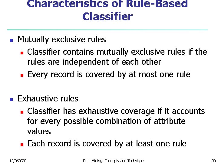
Characteristics of Rule-Based Classifier n n Mutually exclusive rules n Classifier contains mutually exclusive rules if the rules are independent of each other n Every record is covered by at most one rule Exhaustive rules n Classifier has exhaustive coverage if it accounts for every possible combination of attribute values n Each record is covered by at least one rule 12/3/2020 Data Mining: Concepts and Techniques 93

From Decision Trees To Rules are mutually exclusive and exhaustive Rule set contains as much information as the tree 12/3/2020 Data Mining: Concepts and Techniques 94

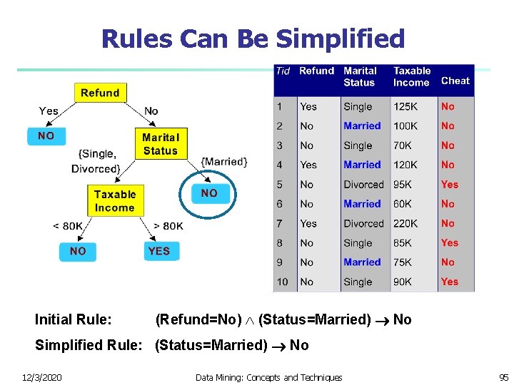
Rules Can Be Simplified Initial Rule: (Refund=No) (Status=Married) No Simplified Rule: (Status=Married) No 12/3/2020 Data Mining: Concepts and Techniques 95

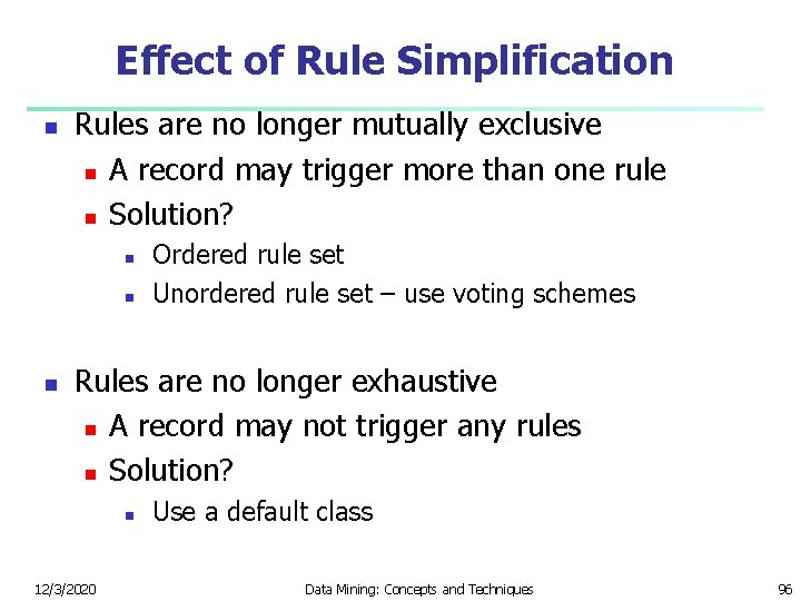
Effect of Rule Simplification n Rules are no longer mutually exclusive n A record may trigger more than one rule n Solution? n n n Ordered rule set Unordered rule set – use voting schemes Rules are no longer exhaustive n A record may not trigger any rules n Solution? n 12/3/2020 Use a default class Data Mining: Concepts and Techniques 96

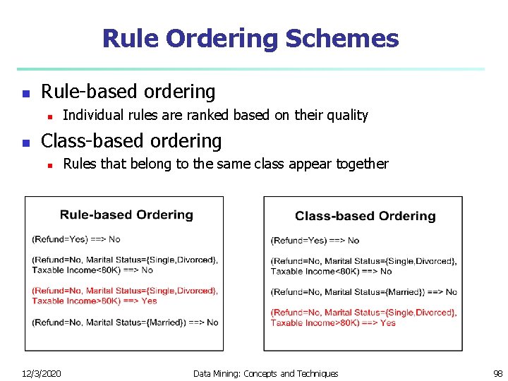
Ordered Rule Set n Rules are rank ordered according to their priority n n An ordered rule set is known as a decision list When a test record is presented to the classifier n n It is assigned to the class label of the highest ranked rule it has triggered If none of the rules fired, it is assigned to the default class R 1: (Give Birth = no) (Can Fly = yes) Birds R 2: (Give Birth = no) (Live in Water = yes) Fishes R 3: (Give Birth = yes) (Blood Type = warm) Mammals R 4: (Give Birth = no) (Can Fly = no) Reptiles R 5: (Live in Water = sometimes) Amphibians 12/3/2020 Data Mining: Concepts and Techniques 97

Rule Ordering Schemes n Rule-based ordering n n Individual rules are ranked based on their quality Class-based ordering n 12/3/2020 Rules that belong to the same class appear together Data Mining: Concepts and Techniques 98

Building Classification Rules n Direct Method: n n n Extract rules directly from data e. g. : RIPPER, CN 2, Holte’s 1 R Indirect Method: n n 12/3/2020 Extract rules from other classification models (e. g. decision trees, neural networks, etc). e. g: C 4. 5 rules Data Mining: Concepts and Techniques 99

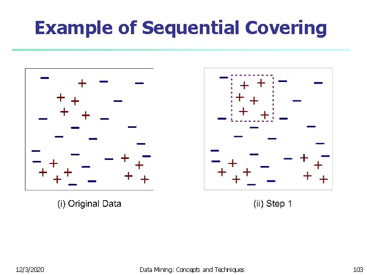
Rule Extraction from the Training Data n Sequential covering algorithm: Extracts rules directly from training data n Typical sequential covering algorithms: FOIL, AQ, CN 2, RIPPER n n Rules are learned sequentially, each for a given class Ci will cover many tuples of Ci but none (or few) of the tuples of other classes Steps: n n Rules are learned one at a time Each time a rule is learned, the tuples covered by the rules are removed The process repeats on the remaining tuples unless termination condition, e. g. , when no more training examples or when the quality of a rule returned is below a user-specified threshold Comp. w. decision-tree induction: learning a set of rules simultaneously 12/3/2020 Data Mining: Concepts and Techniques 100

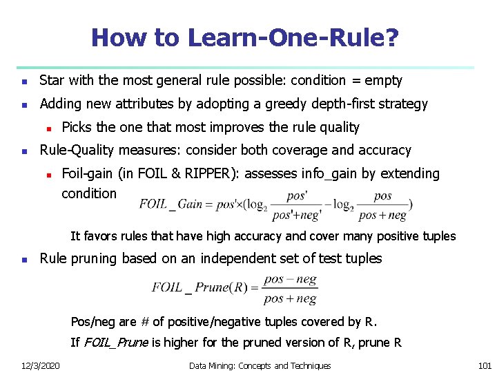
How to Learn-One-Rule? n Star with the most general rule possible: condition = empty n Adding new attributes by adopting a greedy depth-first strategy n n Picks the one that most improves the rule quality Rule-Quality measures: consider both coverage and accuracy n Foil-gain (in FOIL & RIPPER): assesses info_gain by extending condition It favors rules that have high accuracy and cover many positive tuples n Rule pruning based on an independent set of test tuples Pos/neg are # of positive/negative tuples covered by R. If FOIL_Prune is higher for the pruned version of R, prune R 12/3/2020 Data Mining: Concepts and Techniques 101

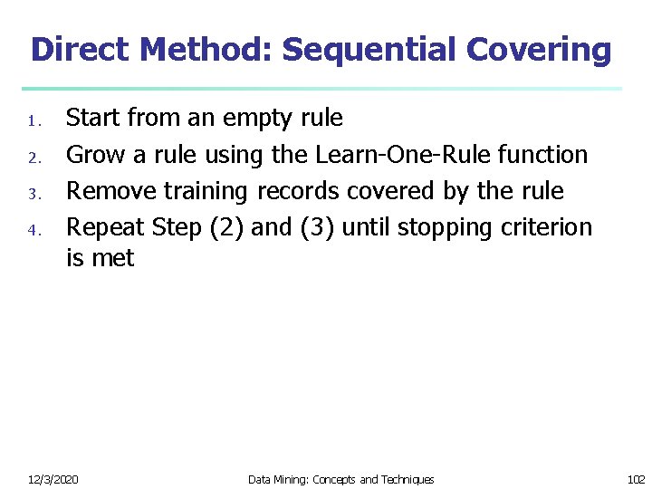
Direct Method: Sequential Covering 1. 2. 3. 4. Start from an empty rule Grow a rule using the Learn-One-Rule function Remove training records covered by the rule Repeat Step (2) and (3) until stopping criterion is met 12/3/2020 Data Mining: Concepts and Techniques 102

Example of Sequential Covering 12/3/2020 Data Mining: Concepts and Techniques 103

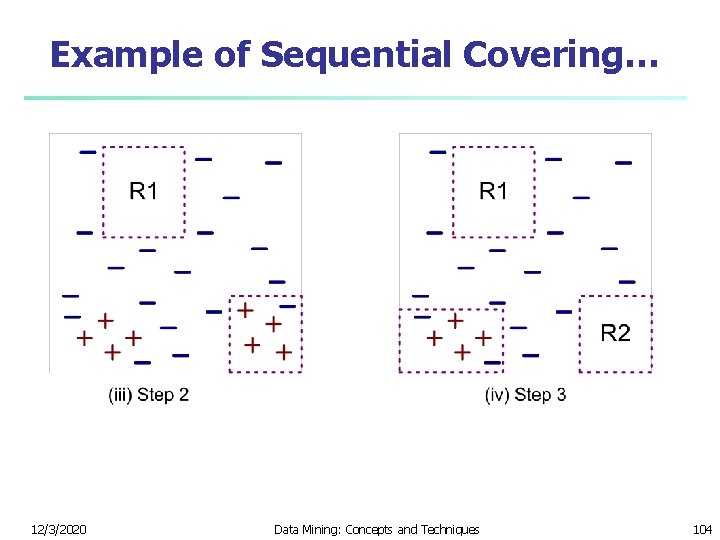
Example of Sequential Covering… 12/3/2020 Data Mining: Concepts and Techniques 104

Aspects of Sequential Covering n Rule Growing n Instance Elimination n Rule Evaluation n Stopping Criterion n Rule Pruning 12/3/2020 Data Mining: Concepts and Techniques 105

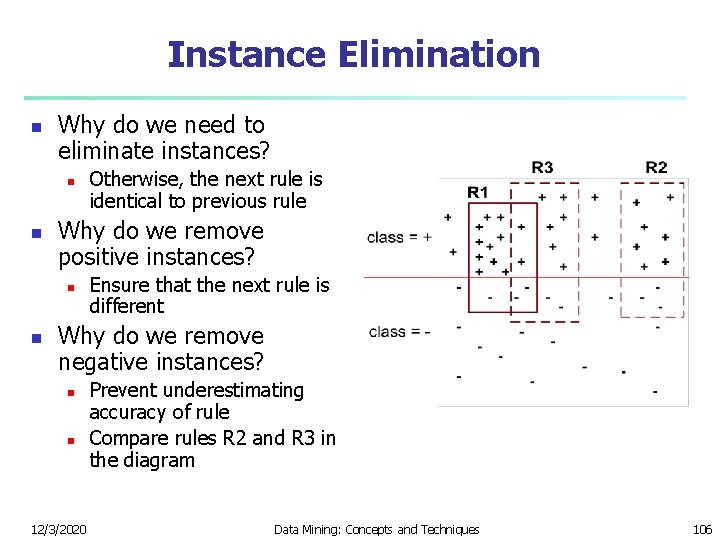
Instance Elimination n Why do we need to eliminate instances? n n Why do we remove positive instances? n n Otherwise, the next rule is identical to previous rule Ensure that the next rule is different Why do we remove negative instances? n n 12/3/2020 Prevent underestimating accuracy of rule Compare rules R 2 and R 3 in the diagram Data Mining: Concepts and Techniques 106

Stopping Criterion and Rule Pruning n n Stopping criterion n Compute the gain n If gain is not significant, discard the new rule Rule Pruning n Similar to post-pruning of decision trees n Reduced Error Pruning: n n n 12/3/2020 Remove one of the conjuncts in the rule Compare error rate on validation set before and after pruning If error improves, prune the conjunct Data Mining: Concepts and Techniques 107

Advantages of Rule-Based Classifiers n n n As highly expressive as decision trees Easy to interpret Easy to generate Can classify new instances rapidly Performance comparable to decision trees 12/3/2020 Data Mining: Concepts and Techniques 108

Chapter 6. Classification and Prediction n n What is classification? What is n Support Vector Machines (SVM) prediction? n Associative classification Issues regarding classification n Lazy learners (or learning from and prediction n your neighbors) Classification by decision tree induction n Bayesian classification n Rule-based classification n Classification by back propagation 12/3/2020 n Other classification methods n Prediction n Accuracy and error measures n Ensemble methods n Model selection n Summary Data Mining: Concepts and Techniques 109

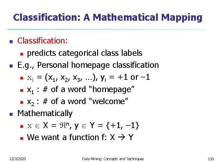
Classification: A Mathematical Mapping n n n Classification: n predicts categorical class labels E. g. , Personal homepage classification n xi = (x 1, x 2, x 3, …), yi = +1 or – 1 n x 1 : # of a word “homepage” n x 2 : # of a word “welcome” Mathematically n n x X = , y Y = {+1, – 1} n We want a function f: X Y 12/3/2020 Data Mining: Concepts and Techniques 110

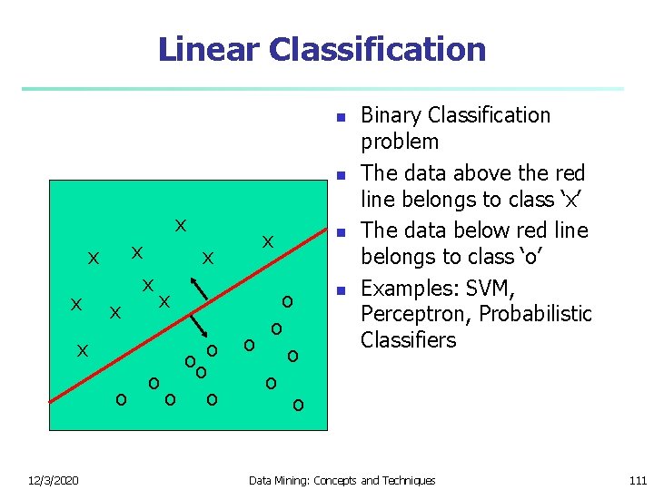
Linear Classification n n x x x 12/3/2020 x x ooo o o x o o o n n Binary Classification problem The data above the red line belongs to class ‘x’ The data below red line belongs to class ‘o’ Examples: SVM, Perceptron, Probabilistic Classifiers Data Mining: Concepts and Techniques 111

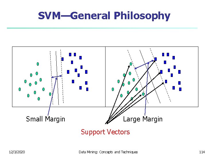
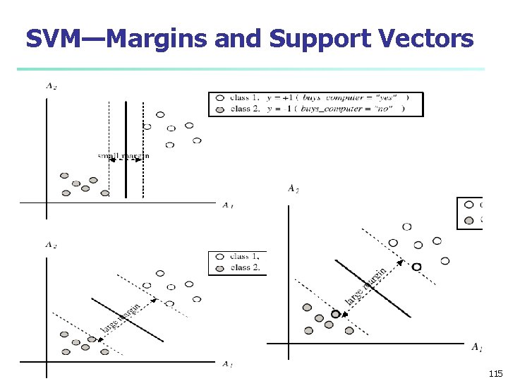
SVM—Support Vector Machines n n n A new classification method for both linear and nonlinear data It uses a nonlinear mapping to transform the original training data into a higher dimension With the new dimension, it searches for the linear optimal separating hyperplane (i. e. , “decision boundary”) With an appropriate nonlinear mapping to a sufficiently high dimension, data from two classes can always be separated by a hyperplane SVM finds this hyperplane using support vectors (“essential” training tuples) and margins (defined by the support vectors) 12/3/2020 Data Mining: Concepts and Techniques 112

SVM—History and Applications n Vapnik and colleagues (1992)—groundwork from Vapnik & Chervonenkis’ statistical learning theory in 1960 s n Features: training can be slow but accuracy is high owing to their ability to model complex nonlinear decision boundaries (margin maximization) n Used both for classification and prediction n Applications: n handwritten digit recognition, object recognition, speaker identification, benchmarking time-series prediction tests 12/3/2020 Data Mining: Concepts and Techniques 113

SVM—General Philosophy Small Margin Large Margin Support Vectors 12/3/2020 Data Mining: Concepts and Techniques 114

SVM—Margins and Support Vectors 12/3/2020 Data Mining: Concepts and Techniques 115

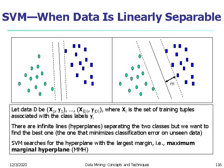
SVM—When Data Is Linearly Separable m Let data D be (X 1, y 1), …, (X|D|, y|D|), where Xi is the set of training tuples associated with the class labels yi There are infinite lines (hyperplanes) separating the two classes but we want to find the best one (the one that minimizes classification error on unseen data) SVM searches for the hyperplane with the largest margin, i. e. , maximum marginal hyperplane (MMH) 12/3/2020 Data Mining: Concepts and Techniques 116

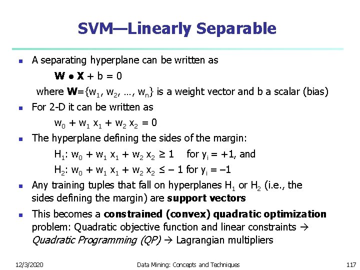
SVM—Linearly Separable n A separating hyperplane can be written as W ● X + b = 0 where W={w 1, w 2, …, wn} is a weight vector and b a scalar (bias) n For 2 -D it can be written as w 0 + w 1 x 1 + w 2 x 2 = 0 n The hyperplane defining the sides of the margin: H 1: w 0 + w 1 x 1 + w 2 x 2 ≥ 1 for yi = +1, and H 2: w 0 + w 1 x 1 + w 2 x 2 ≤ – 1 for yi = – 1 n n Any training tuples that fall on hyperplanes H 1 or H 2 (i. e. , the sides defining the margin) are support vectors This becomes a constrained (convex) quadratic optimization problem: Quadratic objective function and linear constraints Quadratic Programming (QP) Lagrangian multipliers 12/3/2020 Data Mining: Concepts and Techniques 117

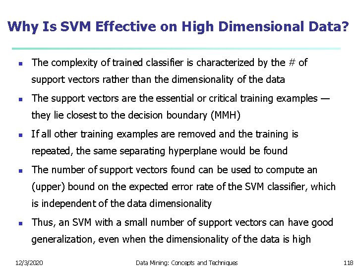
Why Is SVM Effective on High Dimensional Data? n The complexity of trained classifier is characterized by the # of support vectors rather than the dimensionality of the data n The support vectors are the essential or critical training examples — they lie closest to the decision boundary (MMH) n If all other training examples are removed and the training is repeated, the same separating hyperplane would be found n The number of support vectors found can be used to compute an (upper) bound on the expected error rate of the SVM classifier, which is independent of the data dimensionality n Thus, an SVM with a small number of support vectors can have good generalization, even when the dimensionality of the data is high 12/3/2020 Data Mining: Concepts and Techniques 118

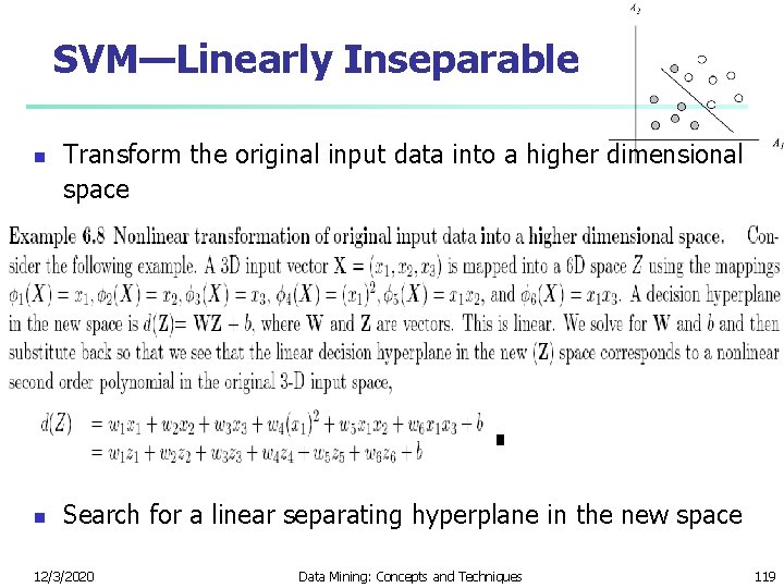
SVM—Linearly Inseparable n n Transform the original input data into a higher dimensional space Search for a linear separating hyperplane in the new space 12/3/2020 Data Mining: Concepts and Techniques 119

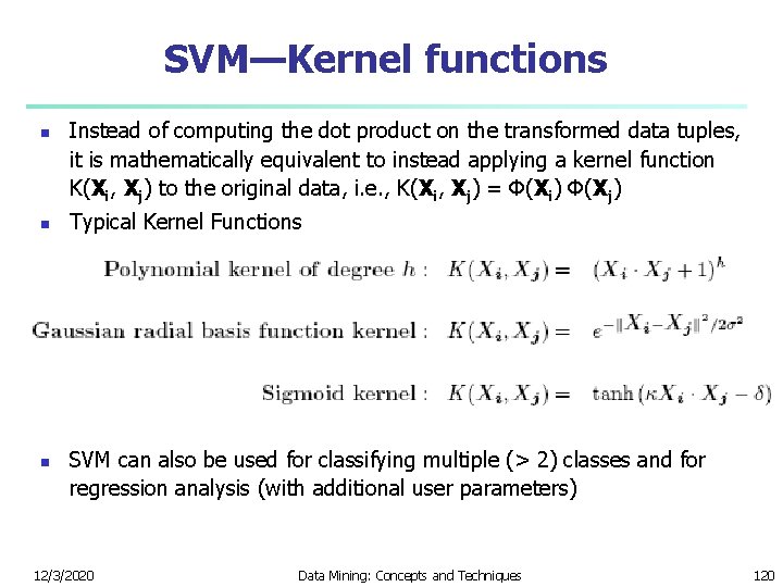
SVM—Kernel functions n n n Instead of computing the dot product on the transformed data tuples, it is mathematically equivalent to instead applying a kernel function K(Xi, Xj) to the original data, i. e. , K(Xi, Xj) = Φ(Xi) Φ(Xj) Typical Kernel Functions SVM can also be used for classifying multiple (> 2) classes and for regression analysis (with additional user parameters) 12/3/2020 Data Mining: Concepts and Techniques 120

SVM—Introduction Literature n “Statistical Learning Theory” by Vapnik: extremely hard to understand, containing many errors too. n C. J. C. Burges. A Tutorial on Support Vector Machines for Pattern Recognition. Knowledge Discovery and Data Mining, 2(2), 1998. n Better than the Vapnik’s book, but still written too hard for introduction, and the examples are so not-intuitive n The book “An Introduction to Support Vector Machines” by N. Cristianini and J. Shawe-Taylor n Also written hard for introduction, but the explanation about the mercer’s theorem is better than above literatures n The neural network book by Haykins n 12/3/2020 Contains one nice chapter of SVM introduction Data Mining: Concepts and Techniques 121