Dimensionality Reduction SVD CUR Mining of Massive Datasets

Dimensionality Reduction: SVD & CUR Mining of Massive Datasets Jure Leskovec, Anand Rajaraman, Jeff Ullman Stanford University Cskh. ir id telegram: @cskh_ir

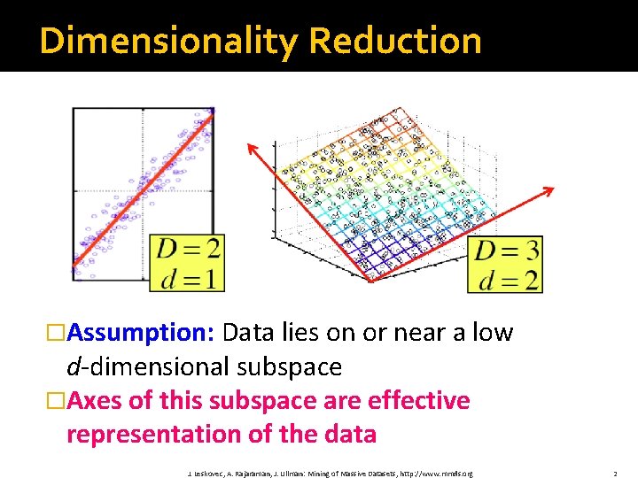
Dimensionality Reduction �Assumption: Data lies on or near a low d‐dimensional subspace �Axes of this subspace are effective representation of the data J. Leskovec, A. Rajaraman, J. Ullman: Mining of Massive Datasets, http: //www. mmds. org 2

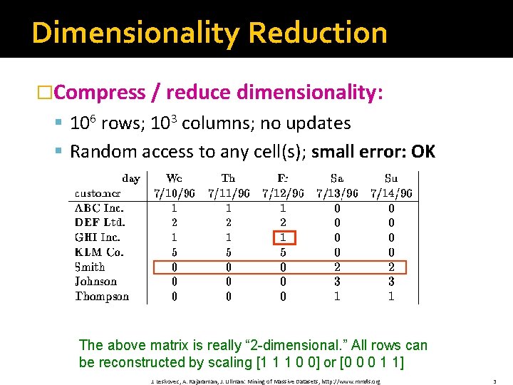
Dimensionality Reduction �Compress / reduce dimensionality: § 106 rows; 103 columns; no updates § Random access to any cell(s); small error: OK The above matrix is really “ 2 -dimensional. ” All rows can be reconstructed by scaling [1 1 1 0 0] or [0 0 0 1 1] J. Leskovec, A. Rajaraman, J. Ullman: Mining of Massive Datasets, http: //www. mmds. org 3

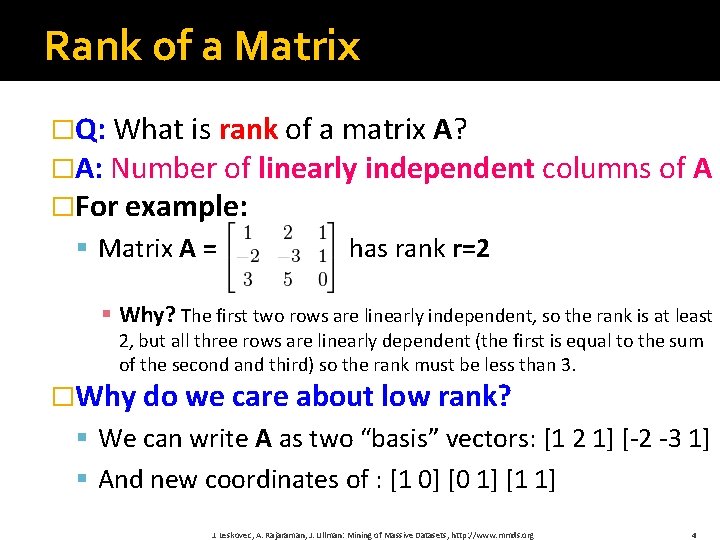
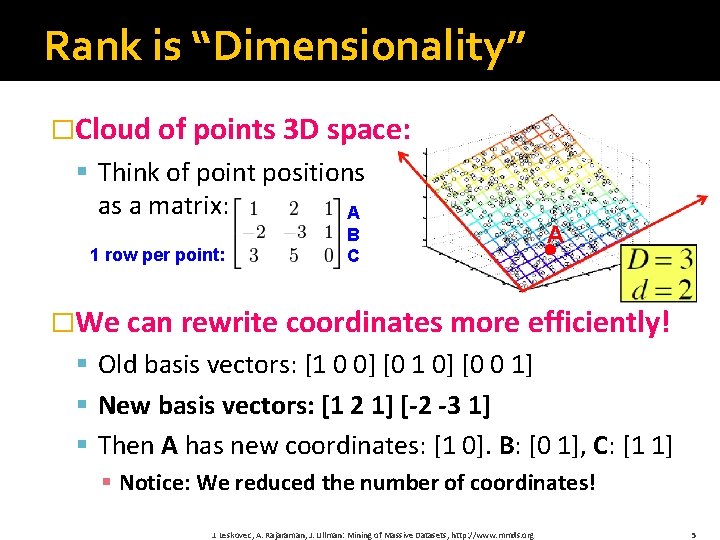
Rank of a Matrix �Q: What is rank of a matrix A? �A: Number of linearly independent columns of A �For example: § Matrix A = has rank r=2 § Why? The first two rows are linearly independent, so the rank is at least 2, but all three rows are linearly dependent (the first is equal to the sum of the second and third) so the rank must be less than 3. �Why do we care about low rank? § We can write A as two “basis” vectors: [1 2 1] [‐ 2 ‐ 3 1] § And new coordinates of : [1 0] [0 1] [1 1] J. Leskovec, A. Rajaraman, J. Ullman: Mining of Massive Datasets, http: //www. mmds. org 4

Rank is “Dimensionality” �Cloud of points 3 D space: § Think of point positions as a matrix: A 1 row per point: B C A �We can rewrite coordinates more efficiently! § Old basis vectors: [1 0 0] [0 1 0] [0 0 1] § New basis vectors: [1 2 1] [-2 -3 1] § Then A has new coordinates: [1 0]. B: [0 1], C: [1 1] § Notice: We reduced the number of coordinates! J. Leskovec, A. Rajaraman, J. Ullman: Mining of Massive Datasets, http: //www. mmds. org 5

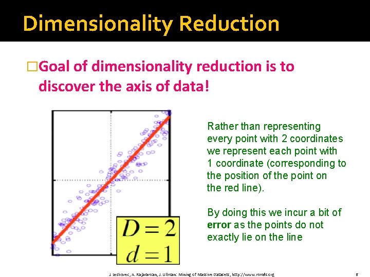
Dimensionality Reduction �Goal of dimensionality reduction is to discover the axis of data! Rather than representing every point with 2 coordinates we represent each point with 1 coordinate (corresponding to the position of the point on the red line). By doing this we incur a bit of error as the points do not exactly lie on the line J. Leskovec, A. Rajaraman, J. Ullman: Mining of Massive Datasets, http: //www. mmds. org 6

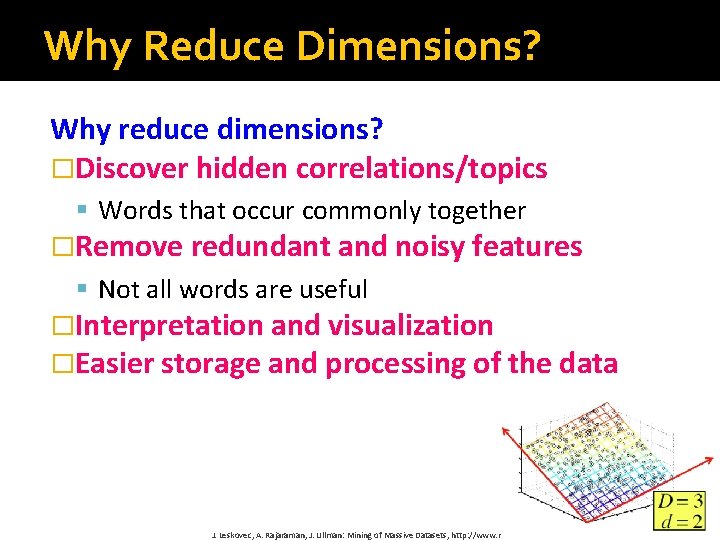
Why Reduce Dimensions? Why reduce dimensions? �Discover hidden correlations/topics § Words that occur commonly together �Remove redundant and noisy features § Not all words are useful �Interpretation and visualization �Easier storage and processing of the data J. Leskovec, A. Rajaraman, J. Ullman: Mining of Massive Datasets, http: //www. mmds. org 7

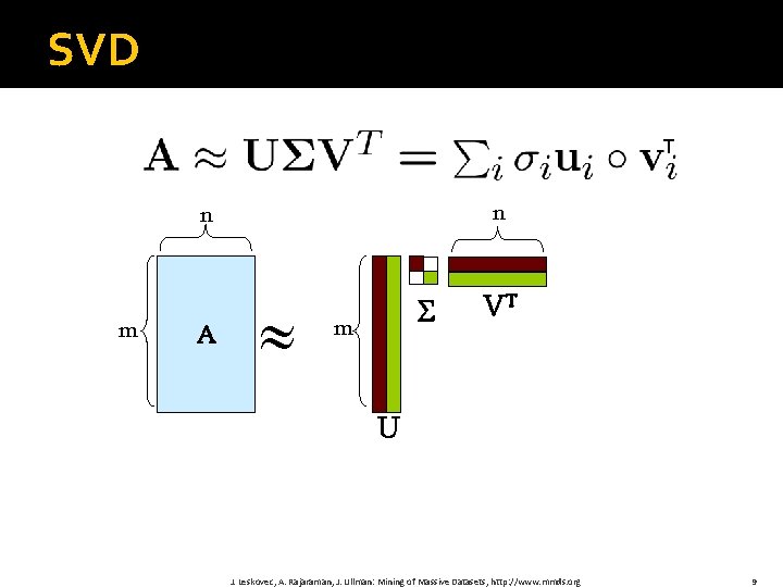
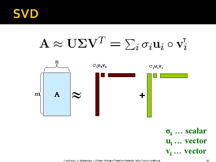
SVD - Definition A[m x n] = U[m x r] [ r x r] (V[n x r])T �A: Input data matrix § m x n matrix (e. g. , m documents, n terms) � U: Left singular vectors § m x r matrix (m documents, r concepts) � : Singular values § r x r diagonal matrix (strength of each ‘concept’) (r : rank of the matrix A) � V: Right singular vectors § n x r matrix (n terms, r concepts) J. Leskovec, A. Rajaraman, J. Ullman: Mining of Massive Datasets, http: //www. mmds. org 8

SVD T n n m A m VT U J. Leskovec, A. Rajaraman, J. Ullman: Mining of Massive Datasets, http: //www. mmds. org 9

SVD T n m A 1 u 1 v 1 2 u 2 v 2 + σi … scalar ui … vector vi … vector J. Leskovec, A. Rajaraman, J. Ullman: Mining of Massive Datasets, http: //www. mmds. org 10

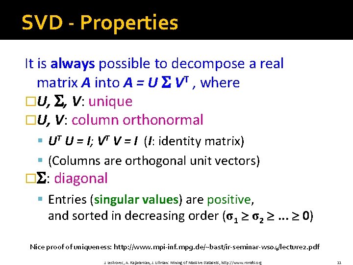
SVD - Properties It is always possible to decompose a real matrix A into A = U VT , where �U, , V: unique �U, V: column orthonormal § UT U = I; VT V = I (I: identity matrix) § (Columns are orthogonal unit vectors) � : diagonal § Entries (singular values) are positive, and sorted in decreasing order (σ1 σ2 . . . 0) Nice proof of uniqueness: http: //www. mpi-inf. mpg. de/~bast/ir-seminar-ws 04/lecture 2. pdf J. Leskovec, A. Rajaraman, J. Ullman: Mining of Massive Datasets, http: //www. mmds. org 11

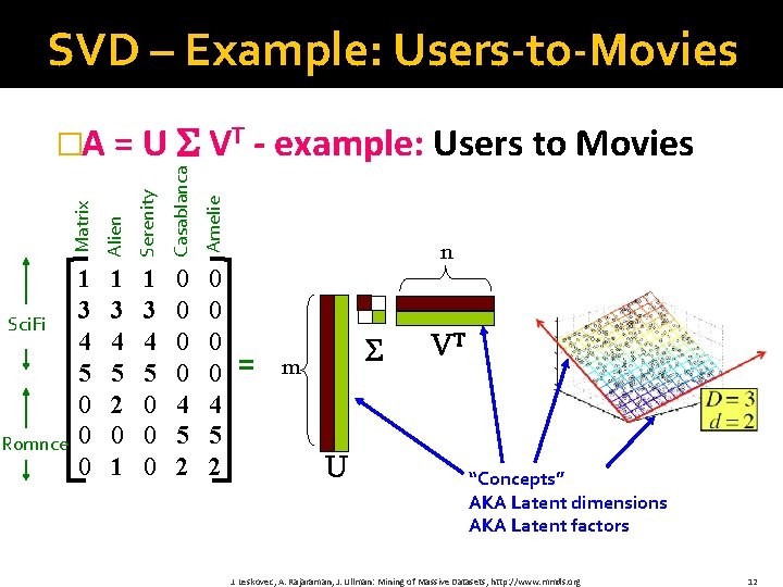
SVD – Example: Users-to-Movies Serenity Casablanca Amelie Romnce Alien Sci. Fi Matrix �A = U VT - example: Users to Movies 1 3 4 5 0 0 0 1 3 4 5 2 0 1 1 3 4 5 0 0 0 0 4 5 2 n = m U VT “Concepts” AKA Latent dimensions AKA Latent factors J. Leskovec, A. Rajaraman, J. Ullman: Mining of Massive Datasets, http: //www. mmds. org 12

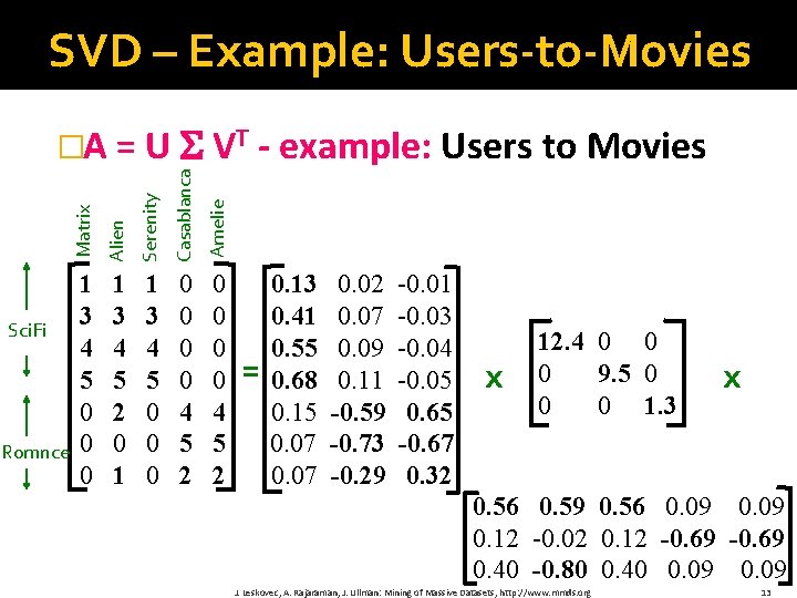
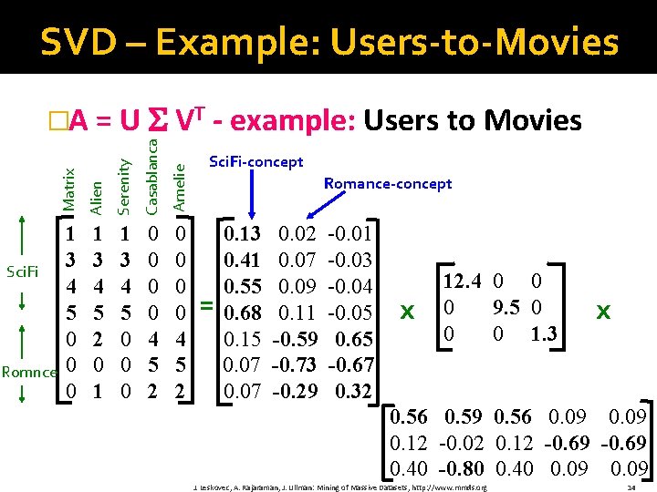
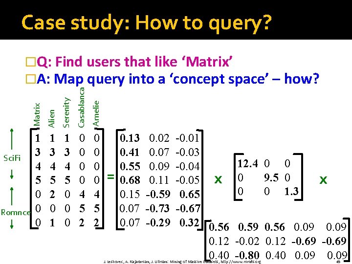
SVD – Example: Users-to-Movies Serenity Casablanca Amelie Romnce Alien Sci. Fi Matrix �A = U VT - example: Users to Movies 1 3 4 5 0 0 0 1 3 4 5 2 0 1 1 3 4 5 0 0 0 0 4 5 2 = 0. 13 0. 41 0. 55 0. 68 0. 15 0. 07 0. 02 0. 07 0. 09 0. 11 -0. 59 -0. 73 -0. 29 -0. 01 -0. 03 -0. 04 -0. 05 0. 65 -0. 67 0. 32 x 12. 4 0 0 0 9. 5 0 0 0 1. 3 x 0. 56 0. 59 0. 56 0. 09 0. 12 -0. 02 0. 12 -0. 69 0. 40 -0. 80 0. 40 0. 09 J. Leskovec, A. Rajaraman, J. Ullman: Mining of Massive Datasets, http: //www. mmds. org 13

SVD – Example: Users-to-Movies Serenity Casablanca Amelie Romnce Alien Sci. Fi Matrix �A = U VT - example: Users to Movies 1 3 4 5 0 0 0 1 3 4 5 2 0 1 1 3 4 5 0 0 0 0 4 5 2 Sci. Fi-concept Romance-concept = 0. 13 0. 41 0. 55 0. 68 0. 15 0. 07 0. 02 0. 07 0. 09 0. 11 -0. 59 -0. 73 -0. 29 -0. 01 -0. 03 -0. 04 -0. 05 0. 65 -0. 67 0. 32 x 12. 4 0 0 0 9. 5 0 0 0 1. 3 x 0. 56 0. 59 0. 56 0. 09 0. 12 -0. 02 0. 12 -0. 69 0. 40 -0. 80 0. 40 0. 09 J. Leskovec, A. Rajaraman, J. Ullman: Mining of Massive Datasets, http: //www. mmds. org 14

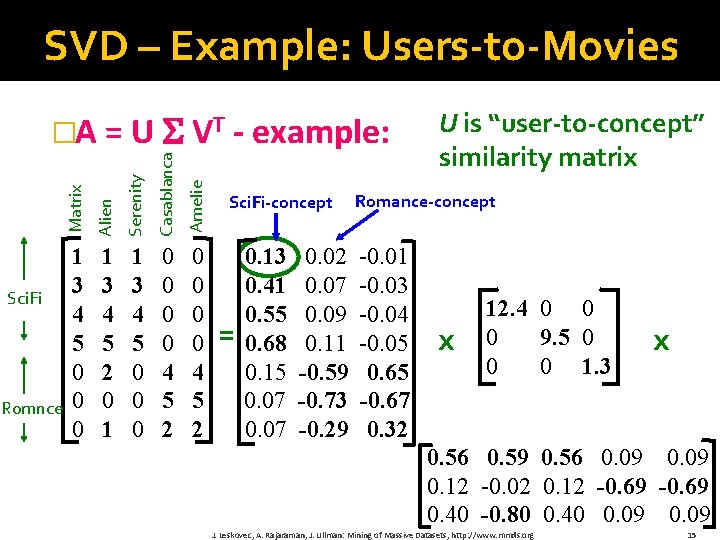
SVD – Example: Users-to-Movies Serenity Casablanca Amelie Romnce Alien Sci. Fi Matrix �A = U VT - example: 1 3 4 5 0 0 0 1 3 4 5 2 0 1 1 3 4 5 0 0 0 0 4 5 2 Sci. Fi-concept = 0. 13 0. 41 0. 55 0. 68 0. 15 0. 07 0. 02 0. 07 0. 09 0. 11 -0. 59 -0. 73 -0. 29 U is “user-to-concept” similarity matrix Romance-concept -0. 01 -0. 03 -0. 04 -0. 05 0. 65 -0. 67 0. 32 x 12. 4 0 0 0 9. 5 0 0 0 1. 3 x 0. 56 0. 59 0. 56 0. 09 0. 12 -0. 02 0. 12 -0. 69 0. 40 -0. 80 0. 40 0. 09 J. Leskovec, A. Rajaraman, J. Ullman: Mining of Massive Datasets, http: //www. mmds. org 15

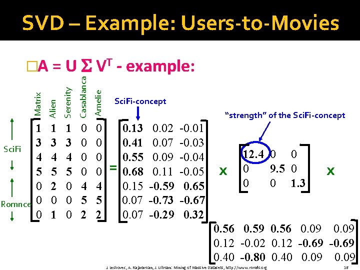
SVD – Example: Users-to-Movies Serenity Casablanca Amelie Romnce Alien Sci. Fi Matrix �A = U VT - example: 1 3 4 5 0 0 0 1 3 4 5 2 0 1 1 3 4 5 0 0 0 0 4 5 2 Sci. Fi-concept “strength” of the Sci. Fi-concept = 0. 13 0. 41 0. 55 0. 68 0. 15 0. 07 0. 02 0. 07 0. 09 0. 11 -0. 59 -0. 73 -0. 29 -0. 01 -0. 03 -0. 04 -0. 05 0. 65 -0. 67 0. 32 x 12. 4 0 0 0 9. 5 0 0 0 1. 3 x 0. 56 0. 59 0. 56 0. 09 0. 12 -0. 02 0. 12 -0. 69 0. 40 -0. 80 0. 40 0. 09 J. Leskovec, A. Rajaraman, J. Ullman: Mining of Massive Datasets, http: //www. mmds. org 16

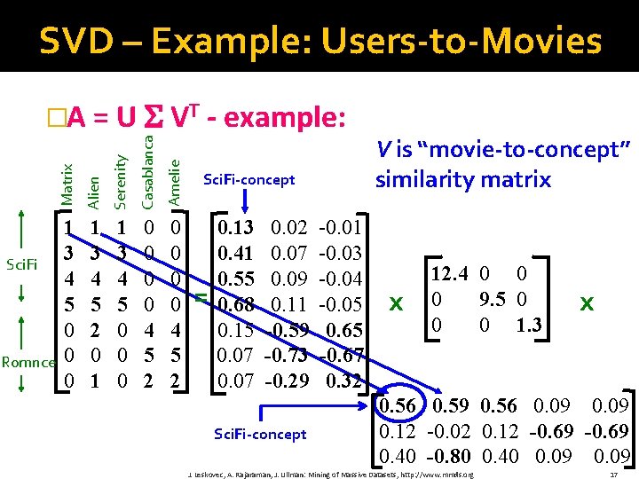
SVD – Example: Users-to-Movies Serenity Casablanca Amelie Romnce Alien Sci. Fi Matrix �A = U VT - example: 1 3 4 5 0 0 0 1 3 4 5 2 0 1 1 3 4 5 0 0 0 0 4 5 2 Sci. Fi-concept = 0. 13 0. 41 0. 55 0. 68 0. 15 0. 07 0. 02 0. 07 0. 09 0. 11 -0. 59 -0. 73 -0. 29 Sci. Fi-concept -0. 01 -0. 03 -0. 04 -0. 05 0. 65 -0. 67 0. 32 V is “movie-to-concept” similarity matrix x 12. 4 0 0 0 9. 5 0 0 0 1. 3 x 0. 56 0. 59 0. 56 0. 09 0. 12 -0. 02 0. 12 -0. 69 0. 40 -0. 80 0. 40 0. 09 J. Leskovec, A. Rajaraman, J. Ullman: Mining of Massive Datasets, http: //www. mmds. org 17

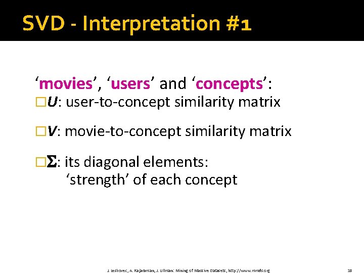
SVD - Interpretation #1 ‘movies’, ‘users’ and ‘concepts’: �U: user‐to‐concept similarity matrix �V: movie‐to‐concept similarity matrix � : its diagonal elements: ‘strength’ of each concept J. Leskovec, A. Rajaraman, J. Ullman: Mining of Massive Datasets, http: //www. mmds. org 18

Dimensionality Reduction with SVD

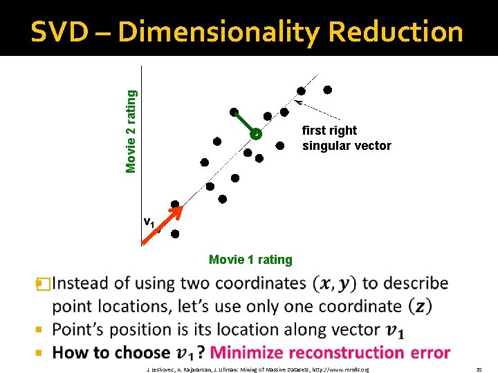
Movie 2 rating SVD – Dimensionality Reduction first right singular vector v 1 Movie 1 rating � J. Leskovec, A. Rajaraman, J. Ullman: Mining of Massive Datasets, http: //www. mmds. org 20

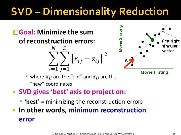
� Movie 2 rating SVD – Dimensionality Reduction first right singular vector v 1 Movie 1 rating J. Leskovec, A. Rajaraman, J. Ullman: Mining of Massive Datasets, http: //www. mmds. org 21

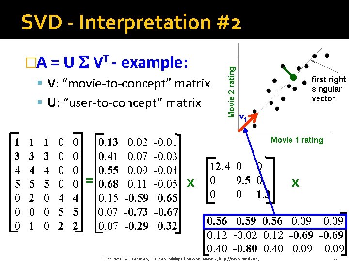
�A = U VT - example: § V: “movie‐to‐concept” matrix § U: “user‐to‐concept” matrix 1 3 4 5 0 0 0 1 3 4 5 2 0 1 1 3 4 5 0 0 0 0 4 5 2 = 0. 13 0. 41 0. 55 0. 68 0. 15 0. 07 0. 02 0. 07 0. 09 0. 11 -0. 59 -0. 73 -0. 29 -0. 01 -0. 03 -0. 04 -0. 05 0. 65 -0. 67 0. 32 Movie 2 rating SVD - Interpretation #2 first right singular vector v 1 Movie 1 rating x 12. 4 0 0 0 9. 5 0 0 0 1. 3 x 0. 56 0. 59 0. 56 0. 09 0. 12 -0. 02 0. 12 -0. 69 0. 40 -0. 80 0. 40 0. 09 J. Leskovec, A. Rajaraman, J. Ullman: Mining of Massive Datasets, http: //www. mmds. org 22

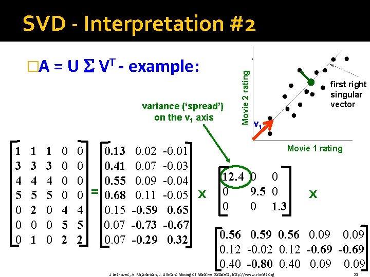
�A = U VT - example: variance (‘spread’) on the v 1 axis 1 3 4 5 0 0 0 1 3 4 5 2 0 1 1 3 4 5 0 0 0 0 4 5 2 = 0. 13 0. 41 0. 55 0. 68 0. 15 0. 07 0. 02 0. 07 0. 09 0. 11 -0. 59 -0. 73 -0. 29 -0. 01 -0. 03 -0. 04 -0. 05 0. 65 -0. 67 0. 32 Movie 2 rating SVD - Interpretation #2 first right singular vector v 1 Movie 1 rating x 12. 4 0 0 0 9. 5 0 0 0 1. 3 x 0. 56 0. 59 0. 56 0. 09 0. 12 -0. 02 0. 12 -0. 69 0. 40 -0. 80 0. 40 0. 09 J. Leskovec, A. Rajaraman, J. Ullman: Mining of Massive Datasets, http: //www. mmds. org 23

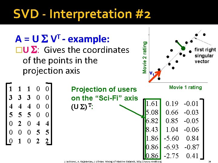
A = U VT - example: �U : Gives the coordinates of the points in the projection axis 1 3 4 5 0 0 0 1 3 4 5 2 0 1 1 3 4 5 0 0 0 0 4 5 2 Projection of users on the “Sci-Fi” axis (U ) T: Movie 2 rating SVD - Interpretation #2 first right singular vector v 1 Movie 1 rating 1. 61 5. 08 6. 82 8. 43 1. 86 0. 86 J. Leskovec, A. Rajaraman, J. Ullman: Mining of Massive Datasets, http: //www. mmds. org 0. 19 0. 66 0. 85 1. 04 -5. 60 -6. 93 -2. 75 -0. 01 -0. 03 -0. 05 -0. 06 0. 84 -0. 87 0. 41 24

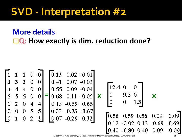
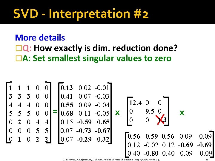
SVD - Interpretation #2 More details �Q: How exactly is dim. reduction done? 1 3 4 5 0 0 0 1 3 4 5 2 0 1 1 3 4 5 0 0 0 0 4 5 2 = 0. 13 0. 41 0. 55 0. 68 0. 15 0. 07 0. 02 0. 07 0. 09 0. 11 -0. 59 -0. 73 -0. 29 -0. 01 -0. 03 -0. 04 -0. 05 0. 65 -0. 67 0. 32 x 12. 4 0 0 0 9. 5 0 0 0 1. 3 x 0. 56 0. 59 0. 56 0. 09 0. 12 -0. 02 0. 12 -0. 69 0. 40 -0. 80 0. 40 0. 09 J. Leskovec, A. Rajaraman, J. Ullman: Mining of Massive Datasets, http: //www. mmds. org 25

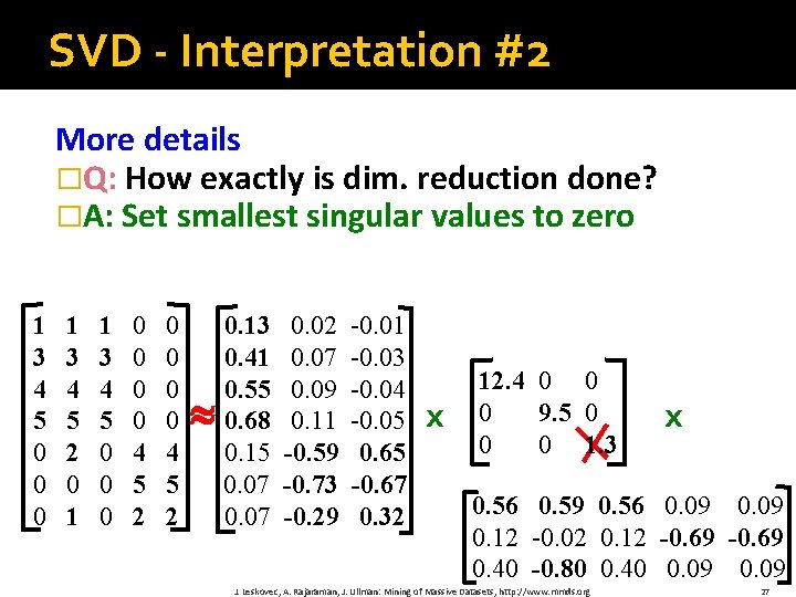
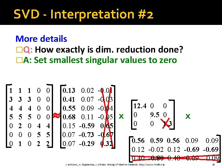
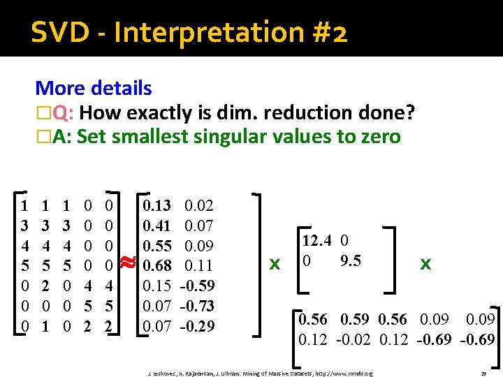
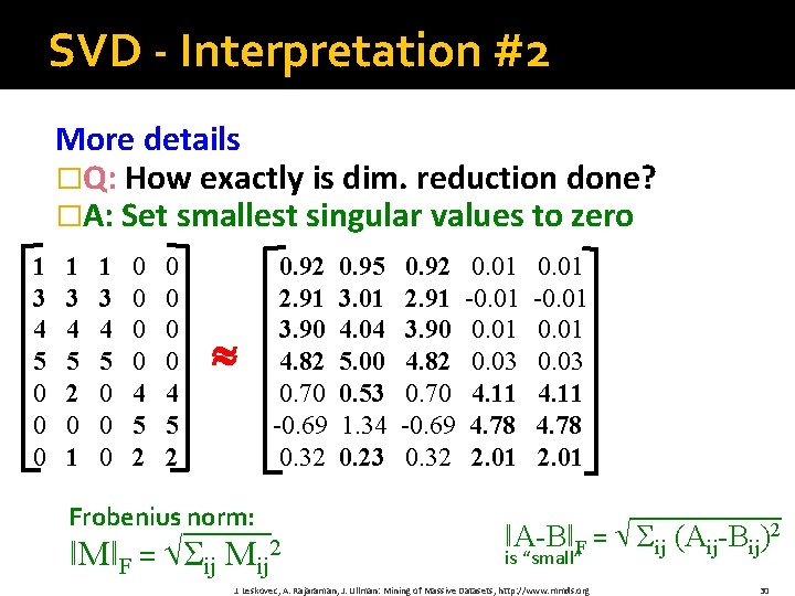
SVD - Interpretation #2 More details �Q: How exactly is dim. reduction done? �A: Set smallest singular values to zero 1 3 4 5 0 0 0 1 3 4 5 2 0 1 1 3 4 5 0 0 0 0 4 5 2 = 0. 13 0. 41 0. 55 0. 68 0. 15 0. 07 0. 02 0. 07 0. 09 0. 11 -0. 59 -0. 73 -0. 29 -0. 01 -0. 03 -0. 04 -0. 05 0. 65 -0. 67 0. 32 x 12. 4 0 0 0 9. 5 0 0 0 1. 3 x 0. 56 0. 59 0. 56 0. 09 0. 12 -0. 02 0. 12 -0. 69 0. 40 -0. 80 0. 40 0. 09 J. Leskovec, A. Rajaraman, J. Ullman: Mining of Massive Datasets, http: //www. mmds. org 26

SVD - Interpretation #2 More details �Q: How exactly is dim. reduction done? �A: Set smallest singular values to zero 1 3 4 5 0 0 0 1 3 4 5 2 0 1 1 3 4 5 0 0 0 0 4 5 2 0. 13 0. 41 0. 55 0. 68 0. 15 0. 07 0. 02 0. 07 0. 09 0. 11 -0. 59 -0. 73 -0. 29 -0. 01 -0. 03 -0. 04 -0. 05 0. 65 -0. 67 0. 32 x 12. 4 0 0 0 9. 5 0 0 0 1. 3 x 0. 56 0. 59 0. 56 0. 09 0. 12 -0. 02 0. 12 -0. 69 0. 40 -0. 80 0. 40 0. 09 J. Leskovec, A. Rajaraman, J. Ullman: Mining of Massive Datasets, http: //www. mmds. org 27

SVD - Interpretation #2 More details �Q: How exactly is dim. reduction done? �A: Set smallest singular values to zero 1 3 4 5 0 0 0 1 3 4 5 2 0 1 1 3 4 5 0 0 0 0 4 5 2 0. 13 0. 41 0. 55 0. 68 0. 15 0. 07 0. 02 0. 07 0. 09 0. 11 -0. 59 -0. 73 -0. 29 -0. 01 -0. 03 -0. 04 -0. 05 0. 65 -0. 67 0. 32 x 12. 4 0 0 0 9. 5 0 0 0 1. 3 x 0. 56 0. 59 0. 56 0. 09 0. 12 -0. 02 0. 12 -0. 69 0. 40 -0. 80 0. 40 0. 09 J. Leskovec, A. Rajaraman, J. Ullman: Mining of Massive Datasets, http: //www. mmds. org 28

SVD - Interpretation #2 More details �Q: How exactly is dim. reduction done? �A: Set smallest singular values to zero 1 3 4 5 0 0 0 1 3 4 5 2 0 1 1 3 4 5 0 0 0 0 4 5 2 0. 13 0. 41 0. 55 0. 68 0. 15 0. 07 0. 02 0. 07 0. 09 0. 11 -0. 59 -0. 73 -0. 29 x 12. 4 0 0 9. 5 x 0. 56 0. 59 0. 56 0. 09 0. 12 -0. 02 0. 12 -0. 69 J. Leskovec, A. Rajaraman, J. Ullman: Mining of Massive Datasets, http: //www. mmds. org 29

SVD - Interpretation #2 More details �Q: How exactly is dim. reduction done? �A: Set smallest singular values to zero 1 3 4 5 0 0 0 1 3 4 5 2 0 1 1 3 4 5 0 0 0 0 4 5 2 Frobenius norm: 0. 92 2. 91 3. 90 4. 82 0. 70 -0. 69 0. 32 ǁMǁF = Σij Mij 2 0. 95 3. 01 4. 04 5. 00 0. 53 1. 34 0. 23 0. 92 2. 91 3. 90 4. 82 0. 70 -0. 69 0. 32 0. 01 -0. 01 0. 03 4. 11 4. 78 2. 01 ǁA-BǁF = Σij (Aij-Bij)2 is “small” J. Leskovec, A. Rajaraman, J. Ullman: Mining of Massive Datasets, http: //www. mmds. org 30

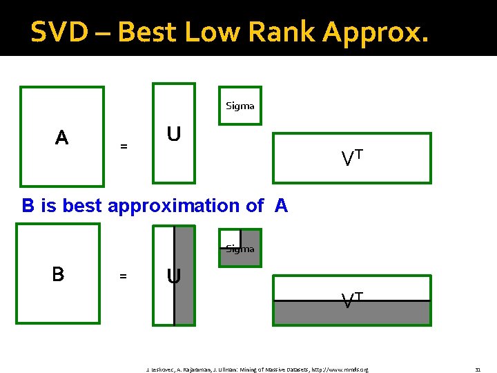
SVD – Best Low Rank Approx. Sigma A = U VT B is best approximation of A Sigma B = U VT J. Leskovec, A. Rajaraman, J. Ullman: Mining of Massive Datasets, http: //www. mmds. org 31

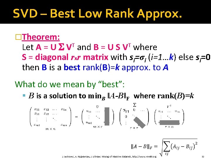
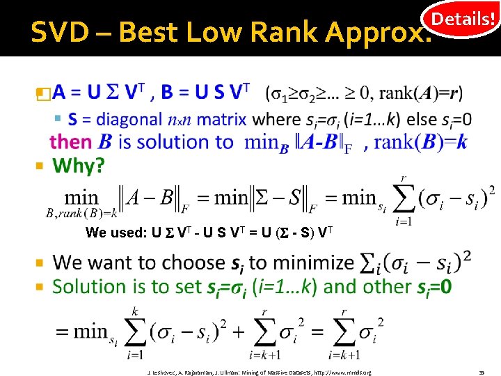
SVD – Best Low Rank Approx. �Theorem: Let A = U VT and B = U S VT where S = diagonal rxr matrix with si=σi (i=1…k) else si=0 then B is a best rank(B)=k approx. to A What do we mean by “best”: § B is a solution to min. B ǁA-BǁF where rank(B)=k J. Leskovec, A. Rajaraman, J. Ullman: Mining of Massive Datasets, http: //www. mmds. org 32

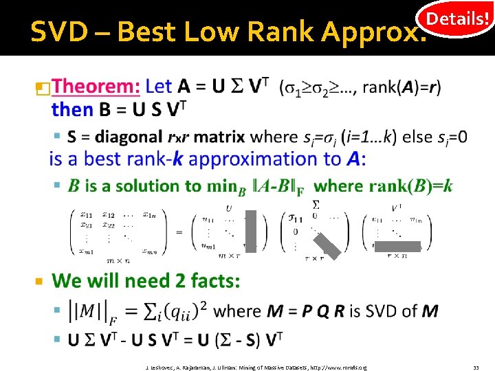
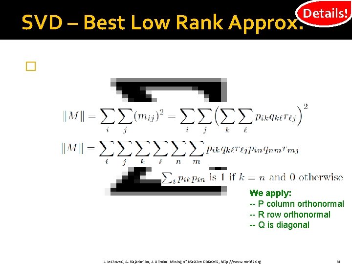
Details! SVD – Best Low Rank Approx. � J. Leskovec, A. Rajaraman, J. Ullman: Mining of Massive Datasets, http: //www. mmds. org 33

Details! SVD – Best Low Rank Approx. � We apply: -- P column orthonormal -- R row orthonormal -- Q is diagonal J. Leskovec, A. Rajaraman, J. Ullman: Mining of Massive Datasets, http: //www. mmds. org 34

Details! SVD – Best Low Rank Approx. � We used: U VT - U S VT = U ( - S) VT J. Leskovec, A. Rajaraman, J. Ullman: Mining of Massive Datasets, http: //www. mmds. org 35

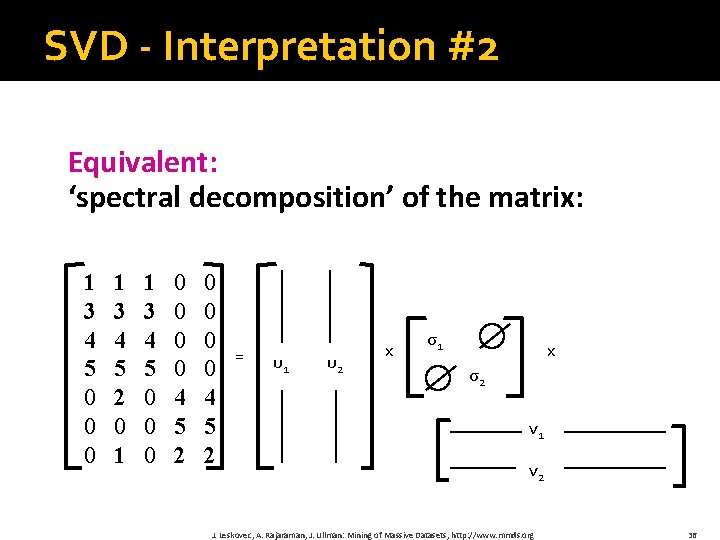
SVD - Interpretation #2 Equivalent: ‘spectral decomposition’ of the matrix: 1 3 4 5 0 0 0 1 3 4 5 2 0 1 1 3 4 5 0 0 0 0 4 5 2 = u 1 u 2 x σ1 x σ2 v 1 v 2 J. Leskovec, A. Rajaraman, J. Ullman: Mining of Massive Datasets, http: //www. mmds. org 36

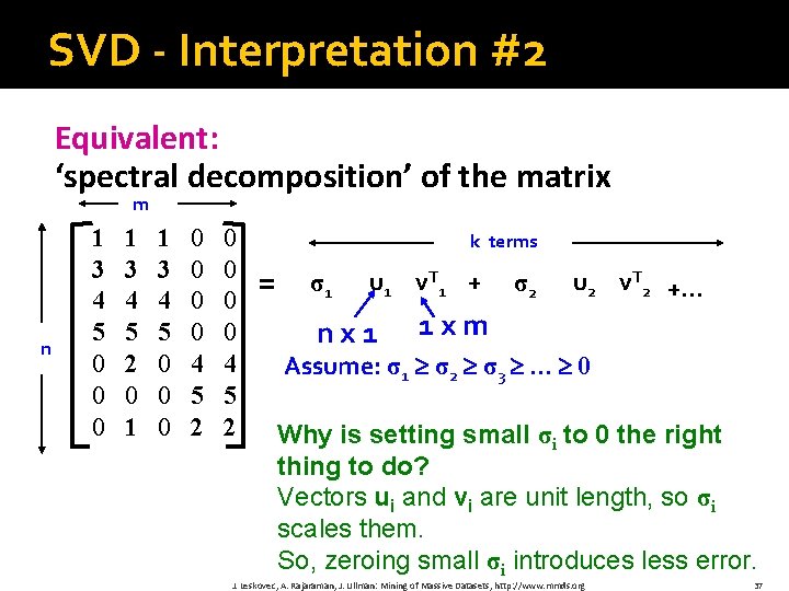
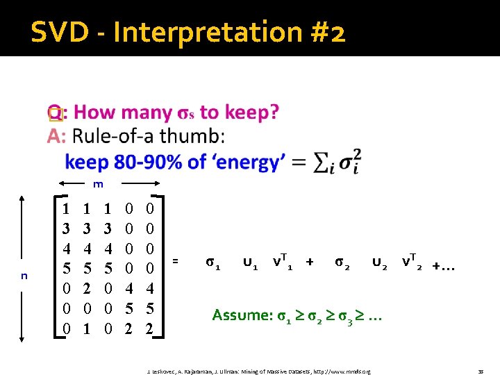
SVD - Interpretation #2 Equivalent: ‘spectral decomposition’ of the matrix m n 1 3 4 5 0 0 0 1 3 4 5 2 0 1 1 3 4 5 0 0 0 0 4 5 2 k terms = σ1 u 1 v. T 1 + nx 1 σ2 u 2 v. T 2 +. . . 1 xm Assume: σ1 σ2 σ3 . . . 0 Why is setting small σi to 0 the right thing to do? Vectors ui and vi are unit length, so σi scales them. So, zeroing small σi introduces less error. J. Leskovec, A. Rajaraman, J. Ullman: Mining of Massive Datasets, http: //www. mmds. org 37

SVD - Interpretation #2 � m n 1 3 4 5 0 0 0 1 3 4 5 2 0 1 1 3 4 5 0 0 0 0 4 5 2 = σ1 u 1 v. T 1 + σ2 u 2 v. T 2 +. . . Assume: σ1 σ2 σ3 . . . J. Leskovec, A. Rajaraman, J. Ullman: Mining of Massive Datasets, http: //www. mmds. org 38

SVD - Complexity �To compute SVD: § O(nm 2) or O(n 2 m) (whichever is less) �But: § Less work, if we just want singular values § or if we want first k singular vectors § or if the matrix is sparse �Implemented in linear algebra packages like § LINPACK, Matlab, SPlus, Mathematica. . . J. Leskovec, A. Rajaraman, J. Ullman: Mining of Massive Datasets, http: //www. mmds. org 39

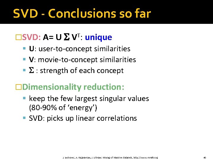
SVD - Conclusions so far �SVD: A= U VT: unique § U: user‐to‐concept similarities § V: movie‐to‐concept similarities § : strength of each concept �Dimensionality reduction: § keep the few largest singular values (80‐ 90% of ‘energy’) § SVD: picks up linear correlations J. Leskovec, A. Rajaraman, J. Ullman: Mining of Massive Datasets, http: //www. mmds. org 40

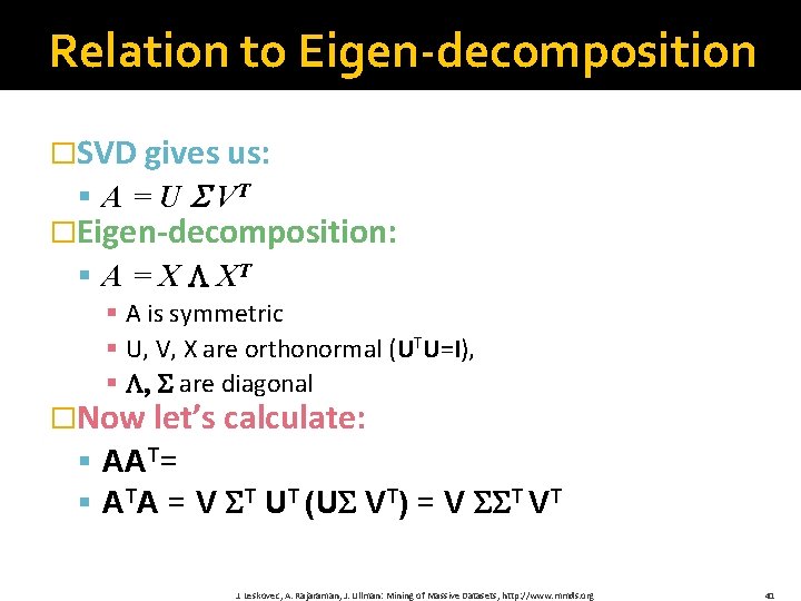
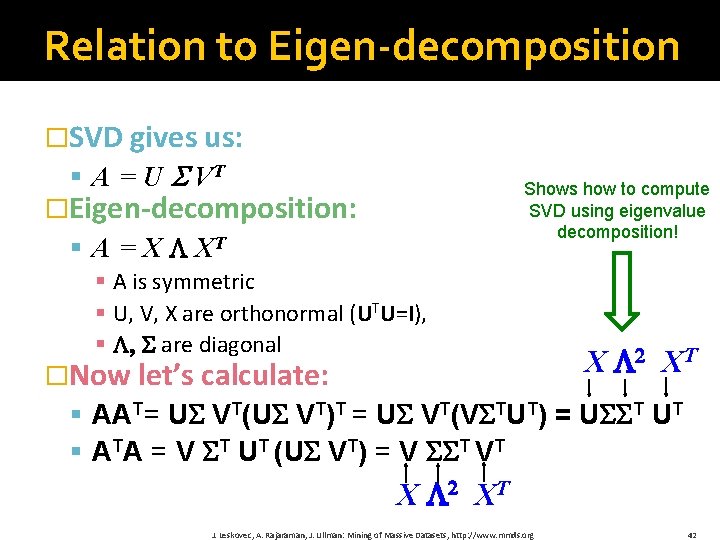
Relation to Eigen-decomposition �SVD gives us: § A = U VT �Eigen-decomposition: § A = X L XT § A is symmetric § U, V, X are orthonormal (UTU=I), § L, are diagonal �Now let’s calculate: § AAT= U VT(U VT)T = U VT(V TUT) = U T UT § ATA = V T UT (U VT) = V T VT J. Leskovec, A. Rajaraman, J. Ullman: Mining of Massive Datasets, http: //www. mmds. org 41

Relation to Eigen-decomposition �SVD gives us: § A = U VT Shows how to compute SVD using eigenvalue decomposition! �Eigen-decomposition: § A = X L XT § A is symmetric § U, V, X are orthonormal (UTU=I), § L, are diagonal �Now let’s calculate: X L 2 X T § AAT= U VT(U VT)T = U VT(V TUT) = U T UT § ATA = V T UT (U VT) = V T VT X L 2 X T J. Leskovec, A. Rajaraman, J. Ullman: Mining of Massive Datasets, http: //www. mmds. org 42

Example of SVD & Conclusion

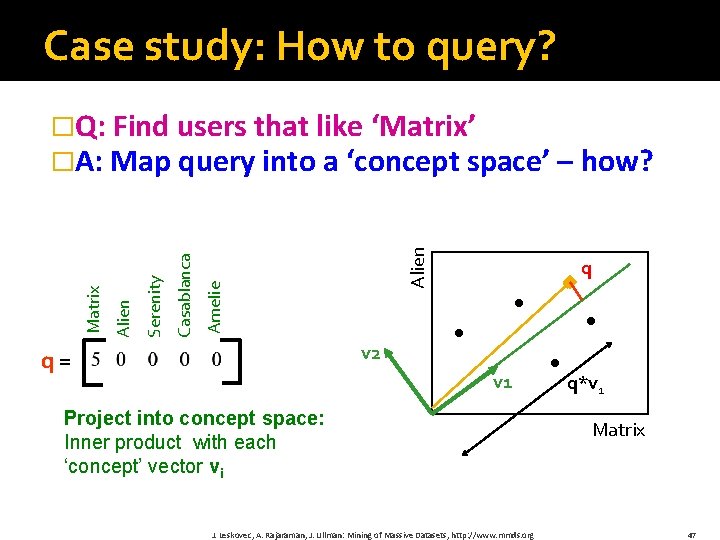
Case study: How to query? Serenity Casablanca Amelie Romnce Alien Sci. Fi Matrix �Q: Find users that like ‘Matrix’ �A: Map query into a ‘concept space’ – how? 1 3 4 5 0 0 0 1 3 4 5 2 0 1 1 3 4 5 0 0 0 0 4 5 2 = 0. 13 0. 41 0. 55 0. 68 0. 15 0. 07 0. 02 0. 07 0. 09 0. 11 -0. 59 -0. 73 -0. 29 -0. 01 -0. 03 -0. 04 -0. 05 x 0. 65 -0. 67 0. 32 0. 56 0. 12 0. 40 12. 4 0 0 0 9. 5 0 0 0 1. 3 x 0. 59 0. 56 0. 09 -0. 02 0. 12 -0. 69 -0. 80 0. 40 0. 09 J. Leskovec, A. Rajaraman, J. Ullman: Mining of Massive Datasets, http: //www. mmds. org 45

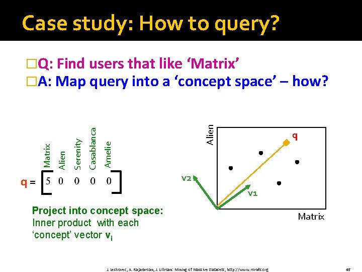
Case study: How to query? Alien Amelie Casablanca Serenity Alien Matrix �Q: Find users that like ‘Matrix’ �A: Map query into a ‘concept space’ – how? q v 2 q = v 1 Project into concept space: Inner product with each ‘concept’ vector vi J. Leskovec, A. Rajaraman, J. Ullman: Mining of Massive Datasets, http: //www. mmds. org Matrix 46

Case study: How to query? Alien Amelie Casablanca Serenity Alien Matrix �Q: Find users that like ‘Matrix’ �A: Map query into a ‘concept space’ – how? q v 2 q = v 1 Project into concept space: Inner product with each ‘concept’ vector vi J. Leskovec, A. Rajaraman, J. Ullman: Mining of Massive Datasets, http: //www. mmds. org q*v 1 Matrix 47

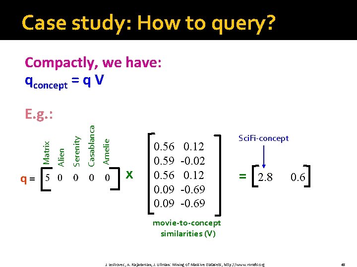
Case study: How to query? Compactly, we have: qconcept = q V q = Amelie Casablanca Serenity Alien Matrix E. g. : x 0. 56 0. 59 0. 56 0. 09 0. 12 -0. 02 0. 12 -0. 69 Sci. Fi-concept = 2. 8 0. 6 movie-to-concept similarities (V) J. Leskovec, A. Rajaraman, J. Ullman: Mining of Massive Datasets, http: //www. mmds. org 48

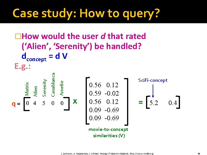
Case study: How to query? �How would the user d that rated q = Amelie Casablanca Serenity Alien Matrix (‘Alien’, ‘Serenity’) be handled? dconcept = d V E. g. : x 0. 56 0. 59 0. 56 0. 09 0. 12 -0. 02 0. 12 -0. 69 Sci. Fi-concept = 5. 2 0. 4 movie-to-concept similarities (V) J. Leskovec, A. Rajaraman, J. Ullman: Mining of Massive Datasets, http: //www. mmds. org 49

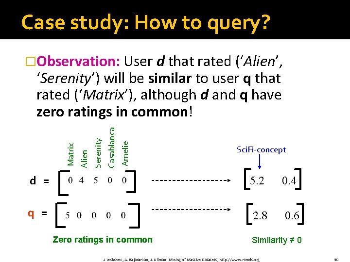
Case study: How to query? �Observation: User d that rated (‘Alien’, Amelie Casablanca Serenity Alien Matrix ‘Serenity’) will be similar to user q that rated (‘Matrix’), although d and q have zero ratings in common! Sci. Fi-concept d = 5. 2 0. 4 q = 2. 8 0. 6 Zero ratings in common Similarity ≠ 0 J. Leskovec, A. Rajaraman, J. Ullman: Mining of Massive Datasets, http: //www. mmds. org 50

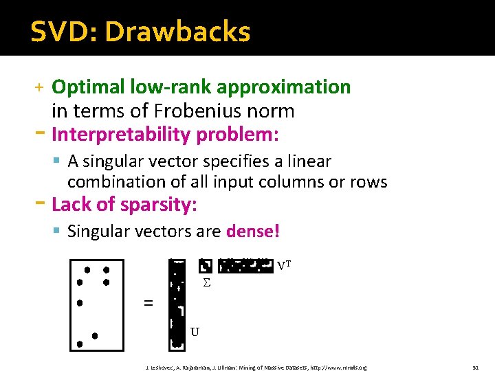
SVD: Drawbacks Optimal low-rank approximation in terms of Frobenius norm - Interpretability problem: + § A singular vector specifies a linear combination of all input columns or rows - Lack of sparsity: § Singular vectors are dense! VT = U J. Leskovec, A. Rajaraman, J. Ullman: Mining of Massive Datasets, http: //www. mmds. org 51

CUR Decomposition

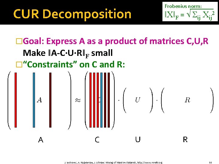
Frobenius norm: CUR Decomposition ǁXǁF = Σij Xij 2 �Goal: Express A as a product of matrices C, U, R Make ǁA-C·U·RǁF small �“Constraints” on C and R: A C U J. Leskovec, A. Rajaraman, J. Ullman: Mining of Massive Datasets, http: //www. mmds. org R 53

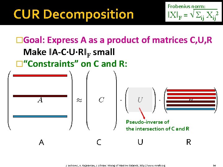
Frobenius norm: CUR Decomposition ǁXǁF = Σij Xij 2 �Goal: Express A as a product of matrices C, U, R Make ǁA-C·U·RǁF small �“Constraints” on C and R: Pseudo-inverse of the intersection of C and R A C U J. Leskovec, A. Rajaraman, J. Ullman: Mining of Massive Datasets, http: //www. mmds. org R 54

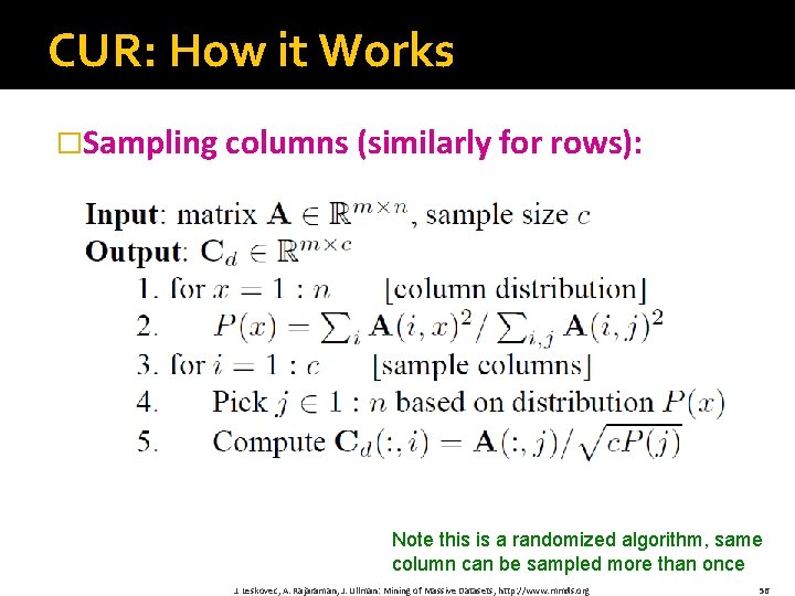
CUR: How it Works �Sampling columns (similarly for rows): Note this is a randomized algorithm, same column can be sampled more than once J. Leskovec, A. Rajaraman, J. Ullman: Mining of Massive Datasets, http: //www. mmds. org 56

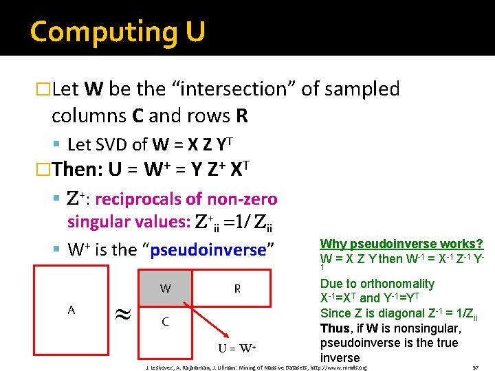
Computing U �Let W be the “intersection” of sampled columns C and rows R § Let SVD of W = X Z YT �Then: U = W+ = Y Z+ XT § Z+: reciprocals of non-zero singular values: Z+ii =1/ Zii § W+ is the “pseudoinverse” Why pseudoinverse works? W = X Z Y then W-1 = X-1 Z-1 Y 1 A W R C U = W+ Due to orthonomality X-1=XT and Y-1=YT Since Z is diagonal Z-1 = 1/Zii Thus, if W is nonsingular, pseudoinverse is the true inverse J. Leskovec, A. Rajaraman, J. Ullman: Mining of Massive Datasets, http: //www. mmds. org 57

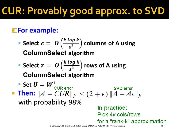
CUR: Provably good approx. to SVD � CUR error SVD error In practice: Pick 4 k cols/rows for a “rank-k” approximation J. Leskovec, A. Rajaraman, J. Ullman: Mining of Massive Datasets, http: //www. mmds. org 58

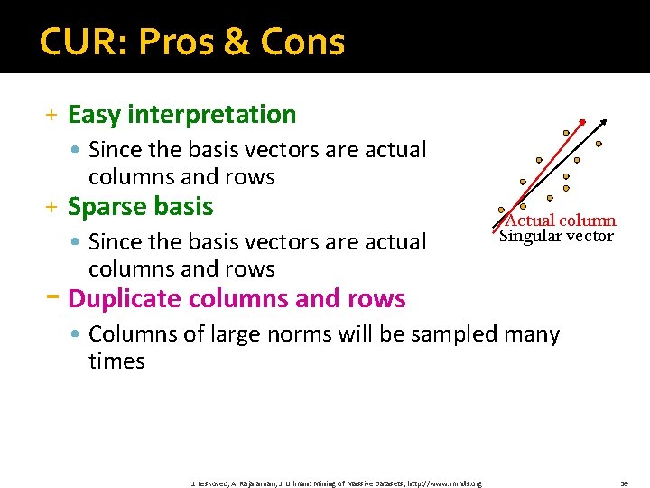
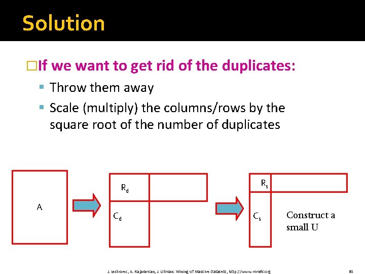
CUR: Pros & Cons + Easy interpretation • Since the basis vectors are actual columns and rows + Sparse basis • Since the basis vectors are actual columns and rows Actual column Singular vector - Duplicate columns and rows • Columns of large norms will be sampled many times J. Leskovec, A. Rajaraman, J. Ullman: Mining of Massive Datasets, http: //www. mmds. org 59

Solution �If we want to get rid of the duplicates: § Throw them away § Scale (multiply) the columns/rows by the square root of the number of duplicates Rd A Cd Rs Cs J. Leskovec, A. Rajaraman, J. Ullman: Mining of Massive Datasets, http: //www. mmds. org Construct a small U 60

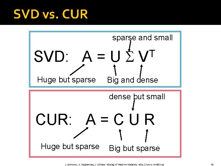
SVD vs. CUR sparse and small SVD: A = U Huge but sparse T V Big and dense but small CUR: A = C U R Huge but sparse Big but sparse J. Leskovec, A. Rajaraman, J. Ullman: Mining of Massive Datasets, http: //www. mmds. org 61

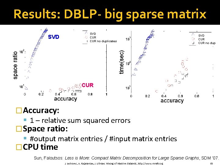
SVD vs. CUR: Simple Experiment �DBLP bibliographic data § Author‐to‐conference big sparse matrix § Aij: Number of papers published by author i at conference j § 428 K authors (rows), 3659 conferences (columns) § Very sparse �Want to reduce dimensionality § How much time does it take? § What is the reconstruction error? § How much space do we need? J. Leskovec, A. Rajaraman, J. Ullman: Mining of Massive Datasets, http: //www. mmds. org 62

Results: DBLP- big sparse matrix SVD CUR no duplicates SVD CUR no dup CUR �Accuracy: § 1 – relative sum squared errors �Space ratio: § #output matrix entries / #input matrix entries �CPU time Sun, Faloutsos: Less is More: Compact Matrix Decomposition for Large Sparse Graphs, SDM ’ 07. J. Leskovec, A. Rajaraman, J. Ullman: Mining of Massive Datasets, http: //www. mmds. org 63

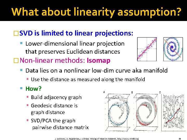
What about linearity assumption? �SVD is limited to linear projections: § Lower‐dimensional linear projection that preserves Euclidean distances �Non‐linear methods: Isomap § Data lies on a nonlinear low‐dim curve aka manifold § Use the distance as measured along the manifold § How? § Build adjacency graph § Geodesic distance is graph distance § SVD/PCA the graph pairwise distance matrix J. Leskovec, A. Rajaraman, J. Ullman: Mining of Massive Datasets, http: //www. mmds. org 64

Further Reading: CUR � Drineas et al. , Fast Monte Carlo Algorithms for Matrices III: Computing a Compressed Approximate Matrix Decomposition, SIAM Journal on Computing, 2006. � J. Sun, Y. Xie, H. Zhang, C. Faloutsos: Less is More: Compact Matrix Decomposition for Large Sparse Graphs, SDM 2007 � Intra- and interpopulation genotype reconstruction from tagging SNPs, P. Paschou, M. W. Mahoney, A. Javed, J. R. Kidd, A. J. Pakstis, S. Gu, K. K. Kidd, and P. Drineas, Genome Research, 17(1), 96‐ 107 (2007) � Tensor-CUR Decompositions For Tensor-Based Data, M. W. Mahoney, M. Maggioni, and P. Drineas, Proc. 12‐th Annual SIGKDD, 327‐ 336 (2006) J. Leskovec, A. Rajaraman, J. Ullman: Mining of Massive Datasets, http: //www. mmds. org 65