Chapter 2 Mining Frequent Patterns Associations and Correlations
![Strong Rules Are Not Necessarily Interesting Buys(X, “computer games”) buys(X, “videos”)[support 40%, confidence=66%] This Strong Rules Are Not Necessarily Interesting Buys(X, “computer games”) buys(X, “videos”)[support 40%, confidence=66%] This](https://slidetodoc.com/presentation_image/8785e028a7b27b27a9237fd49ed0a950/image-44.jpg)
- Slides: 47

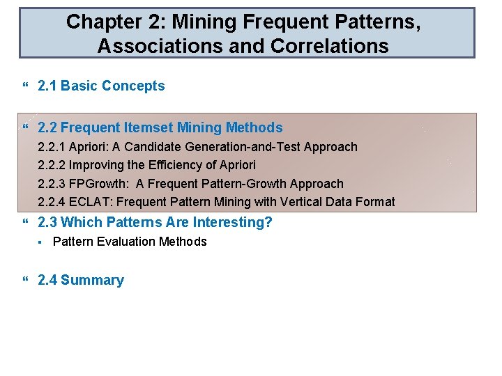
Chapter 2: Mining Frequent Patterns, Associations and Correlations 2. 1 Basic Concepts 2. 2 Frequent Itemset Mining Methods 2. 3 Which Patterns Are Interesting? § Pattern Evaluation Methods 2. 4 Summary

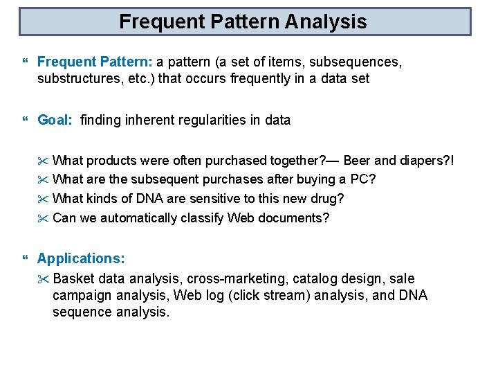
Frequent Pattern Analysis Frequent Pattern: a pattern (a set of items, subsequences, substructures, etc. ) that occurs frequently in a data set Goal: finding inherent regularities in data " What products were often purchased together? — Beer and diapers? ! " What are the subsequent purchases after buying a PC? " What kinds of DNA are sensitive to this new drug? " Can we automatically classify Web documents? Applications: " Basket data analysis, cross-marketing, catalog design, sale campaign analysis, Web log (click stream) analysis, and DNA sequence analysis.

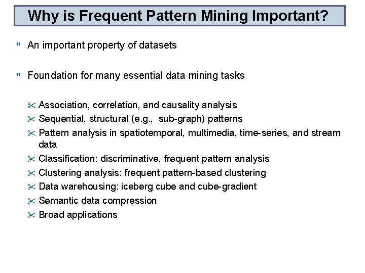
Why is Frequent Pattern Mining Important? An important property of datasets Foundation for many essential data mining tasks " Association, correlation, and causality analysis " Sequential, structural (e. g. , sub-graph) patterns " Pattern analysis in spatiotemporal, multimedia, time-series, and stream data " Classification: discriminative, frequent pattern analysis " Clustering analysis: frequent pattern-based clustering " Data warehousing: iceberg cube and cube-gradient " Semantic data compression " Broad applications

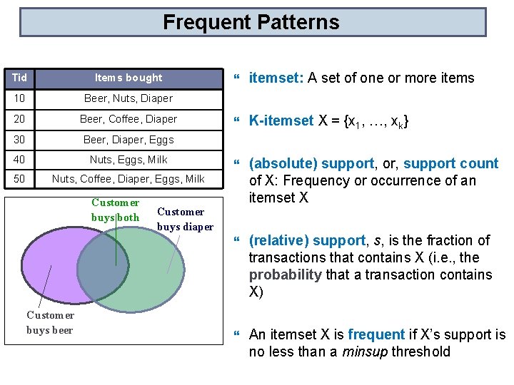
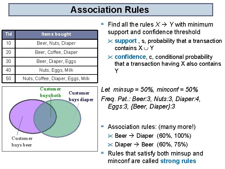
Frequent Patterns Tid Items bought 10 Beer, Nuts, Diaper 20 Beer, Coffee, Diaper 30 Beer, Diaper, Eggs 40 Nuts, Eggs, Milk 50 Nuts, Coffee, Diaper, Eggs, Milk Customer buys both Customer buys beer itemset: A set of one or more items K-itemset X = {x 1, …, xk} (absolute) support, or, support count of X: Frequency or occurrence of an itemset X (relative) support, s, is the fraction of transactions that contains X (i. e. , the probability that a transaction contains X) An itemset X is frequent if X’s support is no less than a minsup threshold Customer buys diaper

Association Rules Tid Items bought 10 Beer, Nuts, Diaper 20 Beer, Coffee, Diaper 30 Beer, Diaper, Eggs 40 Nuts, Eggs, Milk 50 Nuts, Coffee, Diaper, Eggs, Milk Customer buys both Customer buys diaper Find all the rules X Y with minimum support and confidence threshold " support , s, probability that a transaction contains X Y " confidence, c, conditional probability that a transaction having X also contains Y Let minsup = 50%, minconf = 50% Freq. Pat. : Beer: 3, Nuts: 3, Diaper: 4, Eggs: 3, {Beer, Diaper}: 3 Association rules: (many more!) " Beer Diaper (60%, 100%) " Diaper Beer (60%, 75%) Customer buys beer Rules that satisfy both minsup and minconf are called strong rules

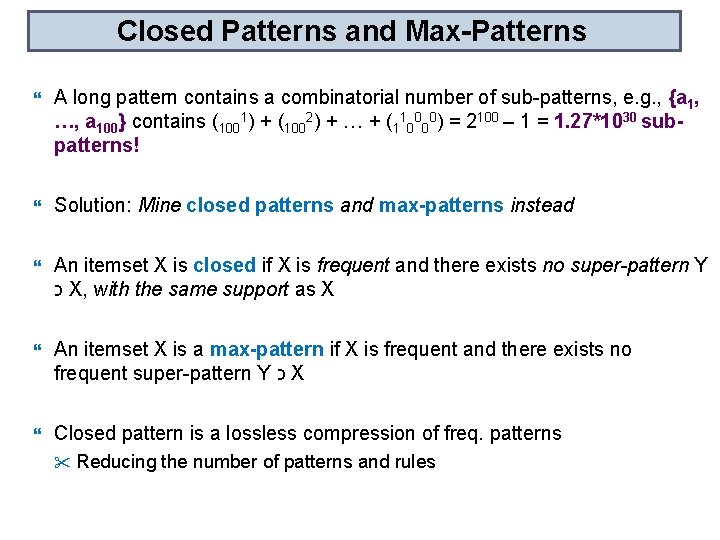
Closed Patterns and Max-Patterns A long pattern contains a combinatorial number of sub-patterns, e. g. , {a 1, …, a 100} contains (1001) + (1002) + … + (110000) = 2100 – 1 = 1. 27*1030 subpatterns! Solution: Mine closed patterns and max-patterns instead An itemset X is closed if X is frequent and there exists no super-pattern Y כ X, with the same support as X An itemset X is a max-pattern if X is frequent and there exists no frequent super-pattern Y כ X Closed pattern is a lossless compression of freq. patterns " Reducing the number of patterns and rules

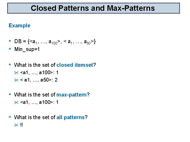
Closed Patterns and Max-Patterns Example DB = {<a 1, …, a 100>, < a 1, …, a 50>} Min_sup=1 What is the set of closed itemset? " <a 1, …, a 100>: 1 " < a 1, …, a 50>: 2 What is the set of max-pattern? " <a 1, …, a 100>: 1 What is the set of all patterns? " !!

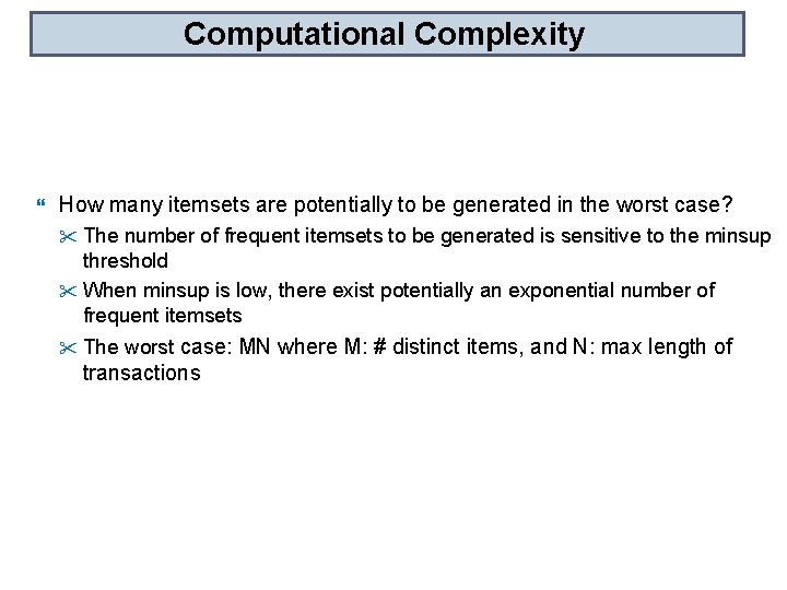
Computational Complexity How many itemsets are potentially to be generated in the worst case? " The number of frequent itemsets to be generated is sensitive to the minsup threshold " When minsup is low, there exist potentially an exponential number of frequent itemsets " The worst case: MN where M: # distinct items, and N: max length of transactions

Chapter 2: Mining Frequent Patterns, Associations and Correlations 2. 1 Basic Concepts 2. 2 Frequent Itemset Mining Methods 2. 2. 1 Apriori: A Candidate Generation-and-Test Approach 2. 2. 2 Improving the Efficiency of Apriori 2. 2. 3 FPGrowth: A Frequent Pattern-Growth Approach 2. 2. 4 ECLAT: Frequent Pattern Mining with Vertical Data Format 2. 3 Which Patterns Are Interesting? § Pattern Evaluation Methods 2. 4 Summary

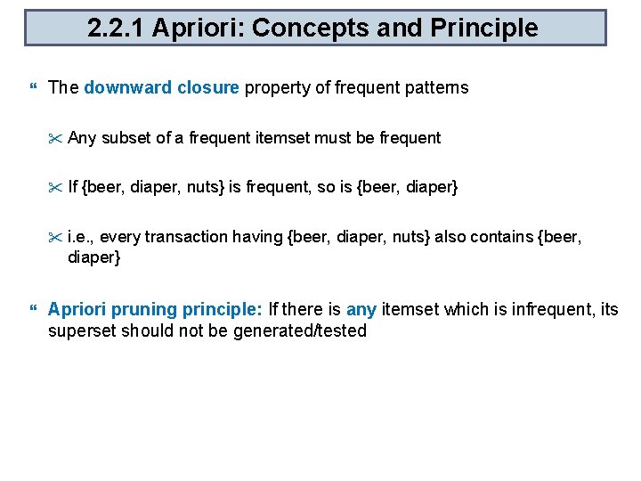
2. 2. 1 Apriori: Concepts and Principle The downward closure property of frequent patterns " Any " If subset of a frequent itemset must be frequent {beer, diaper, nuts} is frequent, so is {beer, diaper} " i. e. , every transaction having {beer, diaper, nuts} also contains {beer, diaper} Apriori pruning principle: If there is any itemset which is infrequent, its superset should not be generated/tested

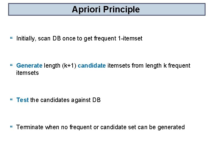
Apriori Principle Initially, scan DB once to get frequent 1 -itemset Generate length (k+1) candidate itemsets from length k frequent itemsets Test the candidates against DB Terminate when no frequent or candidate set can be generated

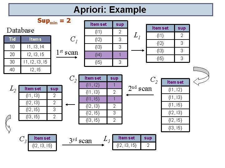
Apriori: Example Supmin = 2 Database Tid Items 10 I 1, I 3, I 4 20 I 2, I 3, I 5 30 I 1, I 2, I 3, I 5 40 I 2, I 5 sup {I 1} 2 {I 2} 3 {I 3} 3 {I 4} 1 {I 5} 3 C 1 1 st scan C 2 L 2 Itemset {I 1, I 3} sup 2 {I 2, I 3} {I 2, I 5} 2 3 {I 3, I 5} 2 Itemset sup {I 1} 2 {I 2} 3 {I 3} 3 {I 5} 3 L 1 Itemset {I 1, I 2} sup 1 {I 1, I 3} {I 1, I 5} 2 1 {I 2, I 3} {I 2, I 5} 2 3 {I 1, I 5} {I 3, I 5} 2 {I 2, I 5} C 2 2 nd scan Itemset {I 1, I 2} {I 1, I 3} {I 2, I 3} {I 3, I 5} C 3 Itemset {I 2, I 3, I 5} 3 rd scan L 3 Itemset sup {I 2, I 3, I 5} 2

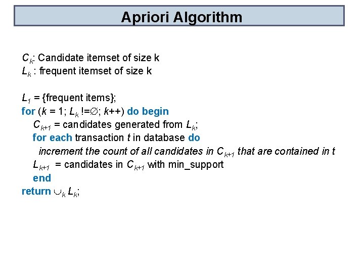
Apriori Algorithm Ck: Candidate itemset of size k Lk : frequent itemset of size k L 1 = {frequent items}; for (k = 1; Lk != ; k++) do begin Ck+1 = candidates generated from Lk; for each transaction t in database do increment the count of all candidates in Ck+1 that are contained in t Lk+1 = candidates in Ck+1 with min_support end return k Lk;

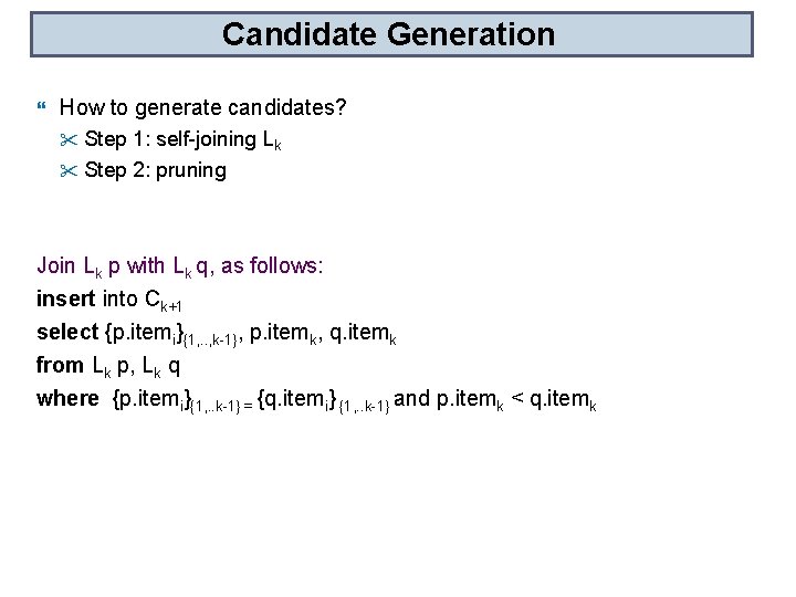
Candidate Generation How to generate candidates? " Step 1: self-joining Lk " Step 2: pruning Join Lk p with Lk q, as follows: insert into Ck+1 select {p. itemi}{1, . . , k-1}, p. itemk, q. itemk from Lk p, Lk q where {p. itemi}{1, . . k-1} = {q. itemi} {1, . . k-1} and p. itemk < q. itemk

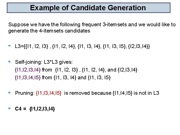
Example of Candidate Generation Suppose we have the following frequent 3 -itemsets and we would like to generate the 4 -itemsets candidates L 3={{I 1, I 2, I 3} , {I 1, I 2, I 4}, {I 1, I 3, I 5}, {I 2, I 3, I 4}} Self-joining: L 3*L 3 gives: {I 1, I 2, I 3, I 4} from {I 1, I 2, I 3} , {I 1, I 2, I 4}, and {I 2, I 3, I 4} {I 1, I 3, I 4, I 5} from {I 1, I 3, I 4} and {I 1, I 3, I 5} Pruning: {I 1, I 3, I 4, I 5} is removed because {I 1, I 4, I 5} is not in L 3 C 4 = {I 1, I 2, I 3, I 4}

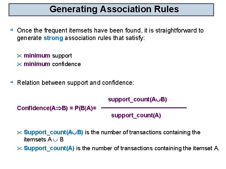
Generating Association Rules Once the frequent itemsets have been found, it is straightforward to generate strong association rules that satisfy: " minimum support " minimum confidence Relation between support and confidence: support_count(A B) Confidence(A B) = P(B|A)= support_count(A) " Support_count(A B) is the number of transactions containing the itemsets A B " Support_count(A) is the number of transactions containing the itemset A.

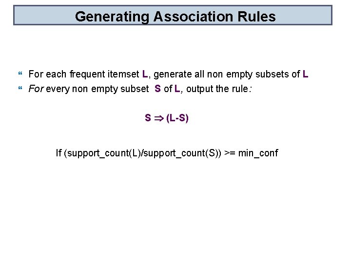
Generating Association Rules For each frequent itemset L, generate all non empty subsets of L For every non empty subset S of L, output the rule: S (L-S) If (support_count(L)/support_count(S)) >= min_conf

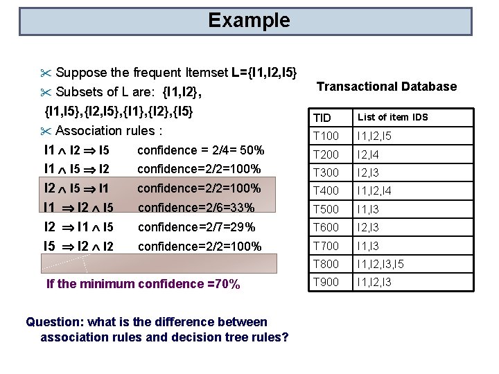
Example " Suppose the frequent Itemset L={I 1, I 2, I 5} " Subsets of L are: {I 1, I 2}, {I 1, I 5}, {I 2, I 5}, {I 1}, {I 2}, {I 5} " Association rules : I 1 I 2 I 5 confidence = 2/4= 50% I 1 I 5 I 2 confidence=2/2=100% I 2 I 5 I 1 confidence=2/2=100% I 1 I 2 I 5 confidence=2/6=33% I 2 I 1 I 5 confidence=2/7=29% I 5 I 2 confidence=2/2=100% If the minimum confidence =70% Question: what is the difference between association rules and decision tree rules? Transactional Database TID List of item IDS T 100 I 1, I 2, I 5 T 200 I 2, I 4 T 300 I 2, I 3 T 400 I 1, I 2, I 4 T 500 I 1, I 3 T 600 I 2, I 3 T 700 I 1, I 3 T 800 I 1, I 2, I 3, I 5 T 900 I 1, I 2, I 3

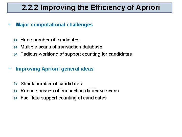
2. 2. 2 Improving the Efficiency of Apriori Major computational challenges " " " Huge number of candidates Multiple scans of transaction database Tedious workload of support counting for candidates Improving Apriori: general ideas " " " Shrink number of candidates Reduce passes of transaction database scans Facilitate support counting of candidates

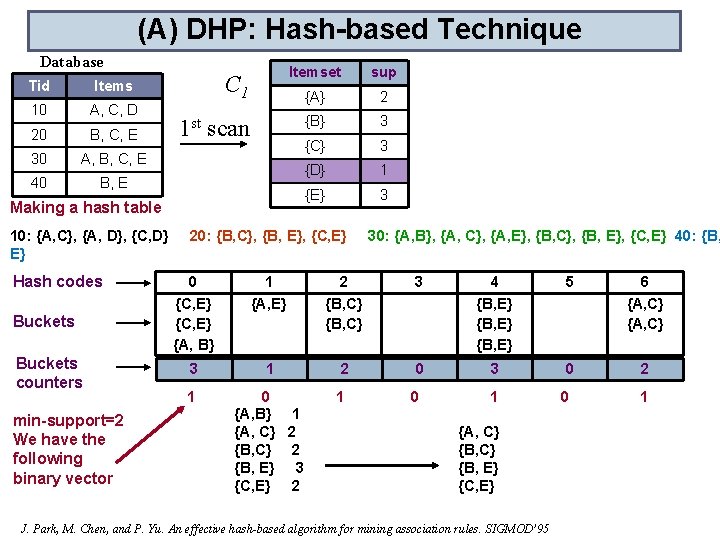
(A) DHP: Hash-based Technique Database Tid Items 10 A, C, D 20 B, C, E 30 A, B, C, E 40 B, E C 1 Itemset sup {A} 2 {B} 3 {C} 3 {D} 1 {E} 3 1 st scan Making a hash table 10: {A, C}, {A, D}, {C, D} E} Hash codes Buckets counters min-support=2 We have the following binary vector 20: {B, C}, {B, E}, {C, E} 30: {A, B}, {A, C}, {A, E}, {B, C}, {B, E}, {C, E} 40: {B, 0 {C, E} {A, B} 1 {A, E} 2 {B, C} 3 4 {B, E} 5 6 {A, C} 3 1 2 0 3 0 2 1 0 {A, B} 1 {A, C} 2 {B, E} 3 {C, E} 2 1 0 1 {A, C} {B, E} {C, E} J. Park, M. Chen, and P. Yu. An effective hash-based algorithm for mining association rules. SIGMOD’ 95 0 1

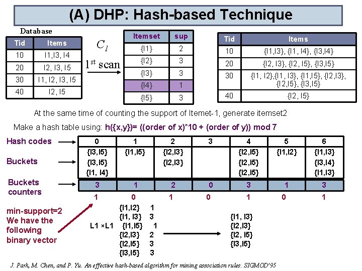
(A) DHP: Hash-based Technique Database Tid Items 10 I 1, I 3, I 4 20 I 2, I 3, I 5 30 I 1, I 2, I 3, I 5 40 I 2, I 5 C 1 Itemset sup Tid Items {I 1} 2 10 {I 1, I 3}, {I 1, I 4}, {I 3, I 4} {I 2} 3 20 {I 2, I 3}, {I 2, I 5}, {I 3, I 5} {I 3} 3 30 {I 4} 1 {I 1, I 2}, {I 1, I 3}, {I 1, I 5}, {I 2, I 3}, {I 2, I 5}, {I 3, I 5} {I 5} 3 40 {I 2, I 5} 1 st scan At the same time of counting the support of Itemet-1, generate itemset 2 Make a hash table using: h({x, y})= ((order of x)*10 + (order of y)) mod 7 Hash codes Buckets counters min-support=2 We have the following binary vector 0 {I 3, I 5} {I 1, I 4} 1 {I 1, I 5} 2 {I 2, I 3} 3 4 {I 2, I 5} 5 {I 1, I 2} 6 {I 1, I 3} {I 3, I 4} {I 1, I 3} 3 1 2 0 3 1 0 {I 1, I 2} {I 1, I 3} L 1 ×L 1 {I 1, I 5} {I 2, I 3} {I 2, I 5} {I 3, I 5} 1 1 3 1 2 3 3 0 1 {I 1, I 3} {I 2, I 5} {I 3, I 5} J. Park, M. Chen, and P. Yu. An effective hash-based algorithm for mining association rules. SIGMOD’ 95 0 1

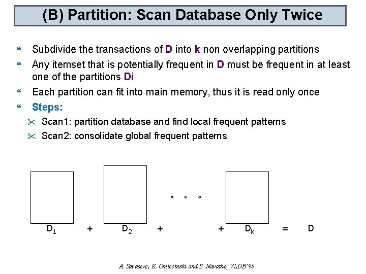
(B) Partition: Scan Database Only Twice Subdivide the transactions of D into k non overlapping partitions Any itemset that is potentially frequent in D must be frequent in at least one of the partitions Di Each partition can fit into main memory, thus it is read only once Steps: " " Scan 1: partition database and find local frequent patterns Scan 2: consolidate global frequent patterns D 1 + D 2 + + Dk A. Savasere, E. Omiecinski and S. Navathe, VLDB’ 95 = D

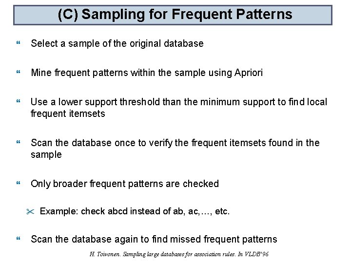
(C) Sampling for Frequent Patterns Select a sample of the original database Mine frequent patterns within the sample using Apriori Use a lower support threshold than the minimum support to find local frequent itemsets Scan the database once to verify the frequent itemsets found in the sample Only broader frequent patterns are checked " Example: check abcd instead of ab, ac, …, etc. Scan the database again to find missed frequent patterns H. Toivonen. Sampling large databases for association rules. In VLDB’ 96

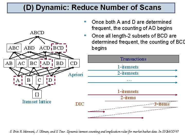
(D) Dynamic: Reduce Number of Scans ABCD ABC ABD ACD BCD AB AC A BC B AD C D {} Itemset lattice BD CD Apriori Once both A and D are determined frequent, the counting of AD begins Once all length-2 subsets of BCD are determined frequent, the counting of BCD begins Transactions 1 -itemsets 2 -itemsets … 1 -itemsets 2 -items DIC 3 -items S. Brin R. Motwani, J. Ullman, and S. Tsur. Dynamic itemset counting and implication rules for market basket data. In SIGMOD’ 97

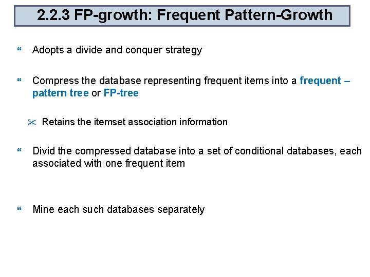
2. 2. 3 FP-growth: Frequent Pattern-Growth Adopts a divide and conquer strategy Compress the database representing frequent items into a frequent – pattern tree or FP-tree " Retains the itemset association information Divid the compressed database into a set of conditional databases, each associated with one frequent item Mine each such databases separately

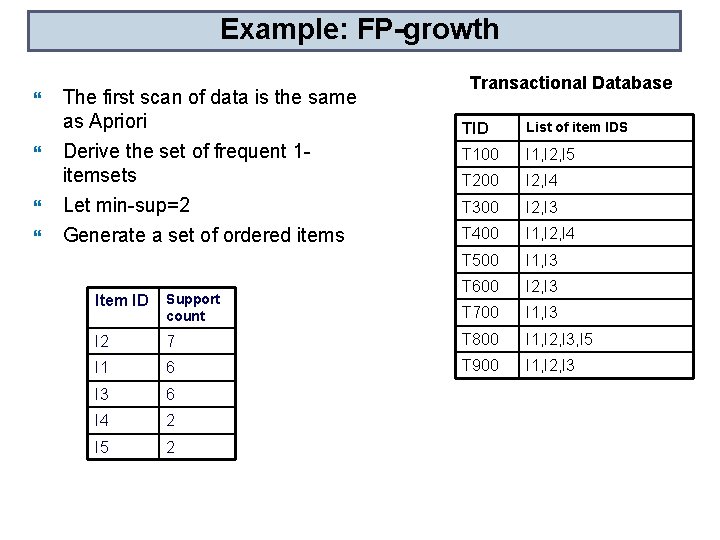
Example: FP-growth The first scan of data is the same as Apriori Derive the set of frequent 1 itemsets Let min-sup=2 Generate a set of ordered items Transactional Database TID List of item IDS T 100 I 1, I 2, I 5 T 200 I 2, I 4 T 300 I 2, I 3 T 400 I 1, I 2, I 4 T 500 I 1, I 3 T 600 I 2, I 3 T 700 I 1, I 3 Item ID Support count I 2 7 T 800 I 1, I 2, I 3, I 5 I 1 6 T 900 I 1, I 2, I 3 6 I 4 2 I 5 2

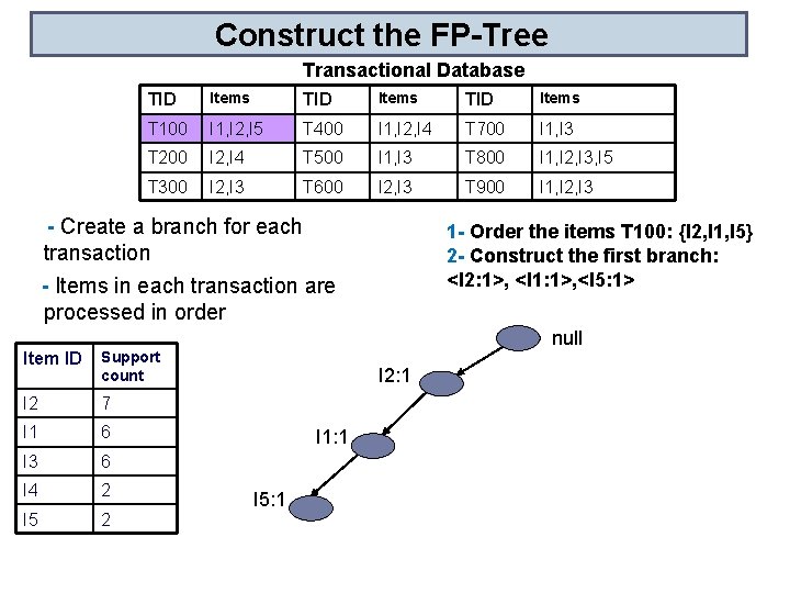
Construct the FP-Tree Transactional Database TID Items T 100 I 1, I 2, I 5 T 400 I 1, I 2, I 4 T 700 I 1, I 3 T 200 I 2, I 4 T 500 I 1, I 3 T 800 I 1, I 2, I 3, I 5 T 300 I 2, I 3 T 600 I 2, I 3 T 900 I 1, I 2, I 3 - Create a branch for each transaction 1 - Order the items T 100: {I 2, I 1, I 5} 2 - Construct the first branch: <I 2: 1>, <I 1: 1>, <I 5: 1> - Items in each transaction are processed in order Item ID Support count I 2 7 I 1 6 I 3 6 I 4 2 I 5 2 null I 2: 1 I 1: 1 I 5: 1

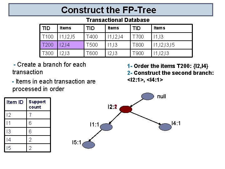
Construct the FP-Tree Transactional Database TID Items T 100 I 1, I 2, I 5 T 400 I 1, I 2, I 4 T 700 I 1, I 3 T 200 I 2, I 4 T 500 I 1, I 3 T 800 I 1, I 2, I 3, I 5 T 300 I 2, I 3 T 600 I 2, I 3 T 900 I 1, I 2, I 3 - Create a branch for each transaction 1 - Order the items T 200: {I 2, I 4} 2 - Construct the second branch: <I 2: 1>, <I 4: 1> - Items in each transaction are processed in order Item ID Support count I 2 7 I 1 6 I 3 6 I 4 2 I 5 2 null I 2: 2 I 2: 1 I 1: 1 I 5: 1 I 4: 1

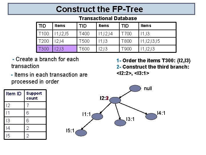
Construct the FP-Tree Transactional Database TID Items T 100 I 1, I 2, I 5 T 400 I 1, I 2, I 4 T 700 I 1, I 3 T 200 I 2, I 4 T 500 I 1, I 3 T 800 I 1, I 2, I 3, I 5 T 300 I 2, I 3 T 600 I 2, I 3 T 900 I 1, I 2, I 3 - Create a branch for each transaction 1 - Order the items T 300: {I 2, I 3} 2 - Construct the third branch: <I 2: 2>, <I 3: 1> - Items in each transaction are processed in order Item ID Support count I 2 7 I 1 6 I 3 6 I 4 2 I 5 2 null I 2: 2 I 2: 3 I 1: 1 I 5: 1 I 4: 1 I 3: 1

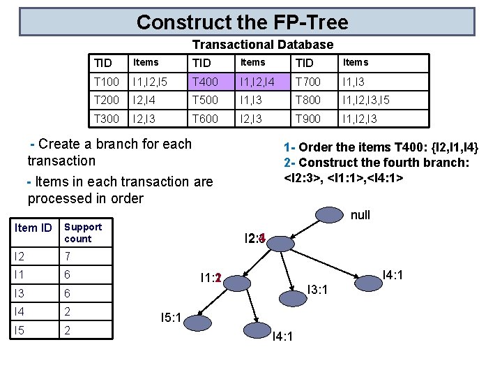
Construct the FP-Tree Transactional Database TID Items T 100 I 1, I 2, I 5 T 400 I 1, I 2, I 4 T 700 I 1, I 3 T 200 I 2, I 4 T 500 I 1, I 3 T 800 I 1, I 2, I 3, I 5 T 300 I 2, I 3 T 600 I 2, I 3 T 900 I 1, I 2, I 3 - Create a branch for each transaction 1 - Order the items T 400: {I 2, I 1, I 4} 2 - Construct the fourth branch: <I 2: 3>, <I 1: 1>, <I 4: 1> - Items in each transaction are processed in order Item ID Support count I 2 7 I 1 6 I 3 6 I 4 2 I 5 2 null I 2: 4 I 2: 3 I 4: 1 I 1: 2 I 1: 1 I 3: 1 I 5: 1 I 4: 1

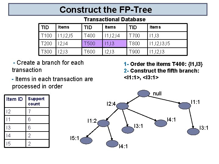
Construct the FP-Tree Transactional Database TID Items T 100 I 1, I 2, I 5 T 400 I 1, I 2, I 4 T 700 I 1, I 3 T 200 I 2, I 4 T 500 I 1, I 3 T 800 I 1, I 2, I 3, I 5 T 300 I 2, I 3 T 600 I 2, I 3 T 900 I 1, I 2, I 3 - Create a branch for each transaction 1 - Order the items T 400: {I 1, I 3} 2 - Construct the fifth branch: <I 1: 1>, <I 3: 1> - Items in each transaction are processed in order Item ID Support count I 2 7 I 1 6 I 3 6 I 4 2 I 5 2 null I 1: 1 I 2: 4 I 4: 1 I 1: 2 I 3: 1 I 5: 1 I 4: 1 I 3: 1

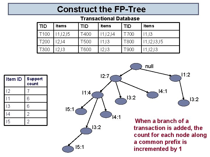
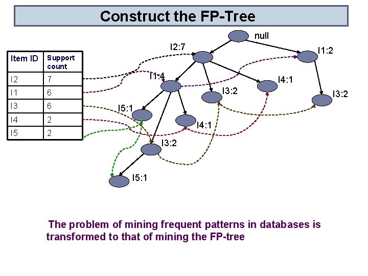
Construct the FP-Tree Transactional Database TID Items T 100 I 1, I 2, I 5 T 400 I 1, I 2, I 4 T 700 I 1, I 3 T 200 I 2, I 4 T 500 I 1, I 3 T 800 I 1, I 2, I 3, I 5 T 300 I 2, I 3 T 600 I 2, I 3 T 900 I 1, I 2, I 3 null Item ID Support count I 2 7 I 1 6 I 3 6 I 4 2 I 5 2 I 1: 2 I 2: 7 I 4: 1 I 1: 4 I 3: 2 I 5: 1 I 4: 1 I 3: 2 I 5: 1 When a branch of a transaction is added, the count for each node along a common prefix is incremented by 1

Construct the FP-Tree null I 2: 7 Item ID Support count I 2 7 I 1 6 I 3 6 I 4 2 I 5 2 I 1: 4 I 4: 1 I 3: 2 I 5: 1 The problem of mining frequent patterns in databases is transformed to that of mining the FP-tree I 3: 2

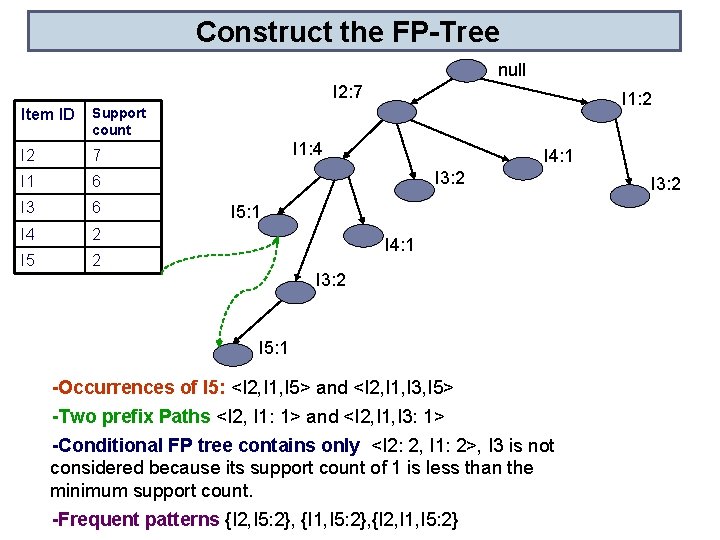
Construct the FP-Tree null I 2: 7 Item ID Support count I 2 7 I 1 6 I 3 6 I 4 2 I 5 2 I 1: 4 I 4: 1 I 3: 2 I 5: 1 -Occurrences of I 5: <I 2, I 1, I 5> and <I 2, I 1, I 3, I 5> -Two prefix Paths <I 2, I 1: 1> and <I 2, I 1, I 3: 1> -Conditional FP tree contains only <I 2: 2, I 1: 2>, I 3 is not considered because its support count of 1 is less than the minimum support count. -Frequent patterns {I 2, I 5: 2}, {I 1, I 5: 2}, {I 2, I 1, I 5: 2} I 3: 2

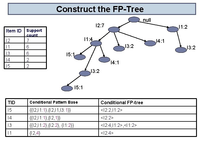
Construct the FP-Tree Item ID Support count I 2 I 1 I 3 I 4 I 5 7 6 6 2 2 null I 2: 7 I 1: 2 I 1: 4 I 3: 2 I 5: 1 I 4: 1 I 3: 2 I 5: 1 TID Conditional Pattern Base Conditional FP-tree I 5 {{I 2, I 1: 1}, {I 2, I 1, I 3: 1}} <I 2: 2, I 1: 2> I 4 {{I 2, I 1: 1}, {I 2, 1}} <I 2: 2> I 3 {{I 2, I 1: 2}, {I 2: 2}, {I 1: 2}} <I 2: 4, I 1: 2>, <I 1: 2> I 1 {I 2, 4} <I 2: 4> I 4: 1 I 3: 2

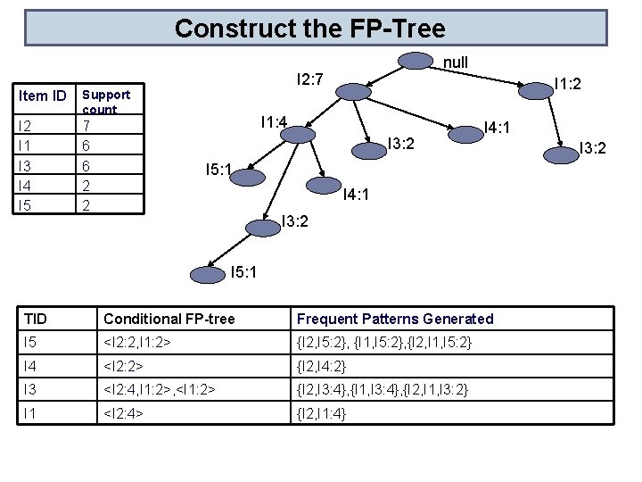
Construct the FP-Tree Item ID Support count I 2 I 1 I 3 I 4 I 5 7 6 6 2 2 null I 2: 7 I 1: 2 I 1: 4 I 3: 2 I 4: 1 I 5: 1 I 4: 1 I 3: 2 I 5: 1 TID Conditional FP-tree Frequent Patterns Generated I 5 <I 2: 2, I 1: 2> {I 2, I 5: 2}, {I 1, I 5: 2}, {I 2, I 1, I 5: 2} I 4 <I 2: 2> {I 2, I 4: 2} I 3 <I 2: 4, I 1: 2>, <I 1: 2> {I 2, I 3: 4}, {I 1, I 3: 4}, {I 2, I 1, I 3: 2} I 1 <I 2: 4> {I 2, I 1: 4} I 3: 2

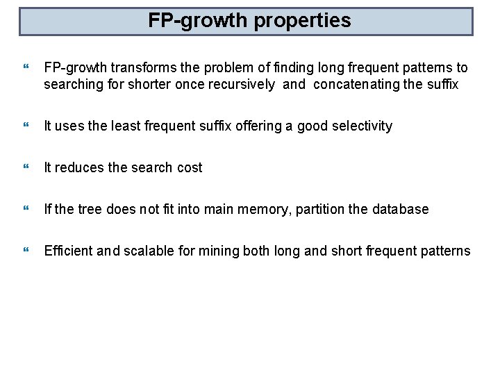
FP-growth properties FP-growth transforms the problem of finding long frequent patterns to searching for shorter once recursively and concatenating the suffix It uses the least frequent suffix offering a good selectivity It reduces the search cost If the tree does not fit into main memory, partition the database Efficient and scalable for mining both long and short frequent patterns

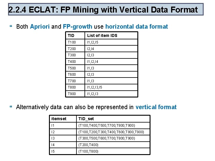
2. 2. 4 ECLAT: FP Mining with Vertical Data Format Both Apriori and FP-growth use horizontal data format TID List of item IDS T 100 I 1, I 2, I 5 T 200 I 2, I 4 T 300 I 2, I 3 T 400 I 1, I 2, I 4 T 500 I 1, I 3 T 600 I 2, I 3 T 700 I 1, I 3 T 800 I 1, I 2, I 3, I 5 T 900 I 1, I 2, I 3 Alternatively data can also be represented in vertical format itemset TID_set I 1 {T 100, T 400, T 500, T 700, T 800, T 900} I 2 {T 100, T 200, T 300, T 400, T 600, T 800, T 900} I 3 {T 300, T 500, T 600, T 700, T 800, T 900} I 4 {T 200, T 400} I 5 {T 100, T 800}

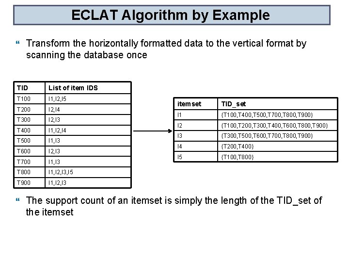
ECLAT Algorithm by Example Transform the horizontally formatted data to the vertical format by scanning the database once TID List of item IDS T 100 I 1, I 2, I 5 T 200 I 2, I 4 T 300 I 2, I 3 T 400 I 1, I 2, I 4 T 500 I 1, I 3 T 600 I 2, I 3 T 700 I 1, I 3 T 800 I 1, I 2, I 3, I 5 T 900 I 1, I 2, I 3 itemset TID_set I 1 {T 100, T 400, T 500, T 700, T 800, T 900} I 2 {T 100, T 200, T 300, T 400, T 600, T 800, T 900} I 3 {T 300, T 500, T 600, T 700, T 800, T 900} I 4 {T 200, T 400} I 5 {T 100, T 800} The support count of an itemset is simply the length of the TID_set of the itemset

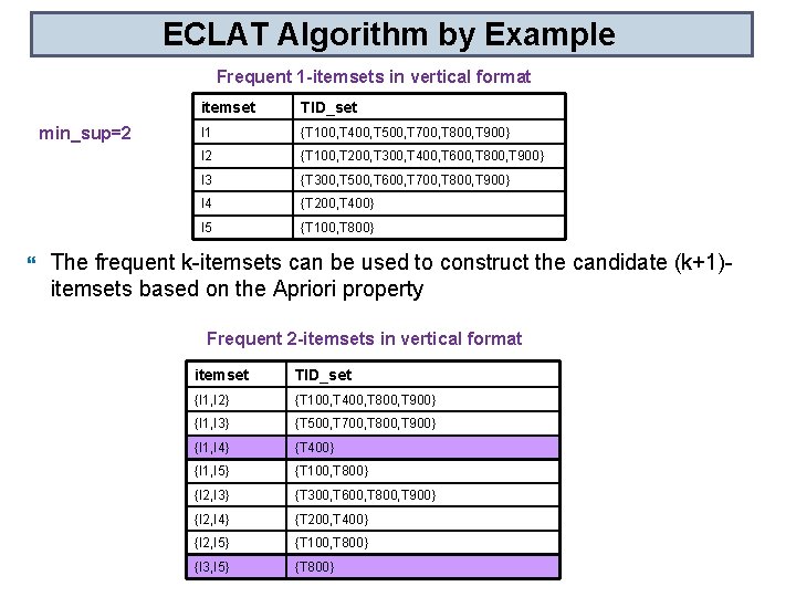
ECLAT Algorithm by Example Frequent 1 -itemsets in vertical format min_sup=2 itemset TID_set I 1 {T 100, T 400, T 500, T 700, T 800, T 900} I 2 {T 100, T 200, T 300, T 400, T 600, T 800, T 900} I 3 {T 300, T 500, T 600, T 700, T 800, T 900} I 4 {T 200, T 400} I 5 {T 100, T 800} The frequent k-itemsets can be used to construct the candidate (k+1)itemsets based on the Apriori property Frequent 2 -itemsets in vertical format itemset TID_set {I 1, I 2} {T 100, T 400, T 800, T 900} {I 1, I 3} {T 500, T 700, T 800, T 900} {I 1, I 4} {T 400} {I 1, I 5} {T 100, T 800} {I 2, I 3} {T 300, T 600, T 800, T 900} {I 2, I 4} {T 200, T 400} {I 2, I 5} {T 100, T 800} {I 3, I 5} {T 800}

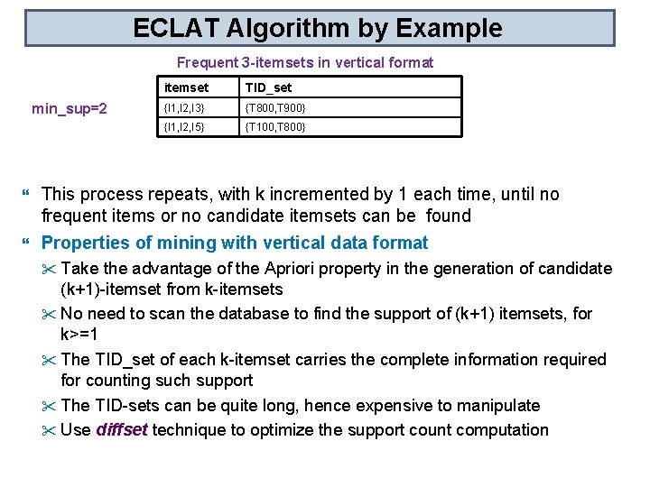
ECLAT Algorithm by Example Frequent 3 -itemsets in vertical format min_sup=2 itemset TID_set {I 1, I 2, I 3} {T 800, T 900} {I 1, I 2, I 5} {T 100, T 800} This process repeats, with k incremented by 1 each time, until no frequent items or no candidate itemsets can be found Properties of mining with vertical data format " Take the advantage of the Apriori property in the generation of candidate (k+1)-itemset from k-itemsets " No need to scan the database to find the support of (k+1) itemsets, for k>=1 " The TID_set of each k-itemset carries the complete information required for counting such support " The TID-sets can be quite long, hence expensive to manipulate " Use diffset technique to optimize the support count computation

Chapter 2: Mining Frequent Patterns, Associations and Correlations 2. 1 Basic Concepts 2. 2 Frequent Itemset Mining Methods 2. 2. 1 Apriori: A Candidate Generation-and-Test Approach 2. 2. 2 Improving the Efficiency of Apriori 2. 2. 3 FPGrowth: A Frequent Pattern-Growth Approach 2. 2. 4 ECLAT: Frequent Pattern Mining with Vertical Data Format 2. 3 Which Patterns Are Interesting? § Pattern Evaluation Methods 2. 4 Summary

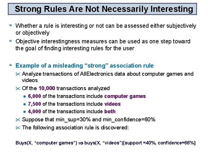
Strong Rules Are Not Necessarily Interesting Whether a rule is interesting or not can be assessed either subjectively or objectively Objective interestingness measures can be used as one step toward the goal of finding interesting rules for the user Example of a misleading “strong” association rule " Analyze transactions of All. Electronics data about computer games and videos " Of the 10, 000 transactions analyzed 6, 000 of the transactions include computer games 7, 500 of the transactions include videos 4, 000 of the transactions include both " Suppose that min_sup=30% and min_confidence=60% " The following association rule is discovered: Buys(X, “computer games”) buys(X, “videos”)[support =40%, confidence=66%]
![Strong Rules Are Not Necessarily Interesting BuysX computer games buysX videossupport 40 confidence66 This Strong Rules Are Not Necessarily Interesting Buys(X, “computer games”) buys(X, “videos”)[support 40%, confidence=66%] This](https://slidetodoc.com/presentation_image/8785e028a7b27b27a9237fd49ed0a950/image-44.jpg)
Strong Rules Are Not Necessarily Interesting Buys(X, “computer games”) buys(X, “videos”)[support 40%, confidence=66%] This rule is strong but it is misleading The probability of purshasing videos is 75% which is even larger than 66% In fact computer games and videos are negatively associated because the purchase of one of these items actually decreases the likelihood of purchasing the other The confidence of a rule A B can be deceiving " It is only an estimate of the conditional probability of itemset B given itemset A. " It does not measure the real strength of the correlation implication between A and B Need to use Correlation Analysis

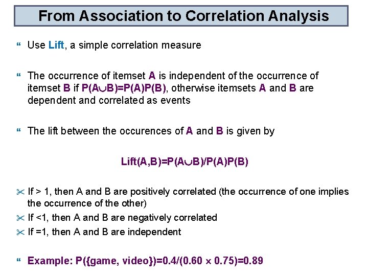
From Association to Correlation Analysis Use Lift, a simple correlation measure The occurrence of itemset A is independent of the occurrence of itemset B if P(A B)=P(A)P(B), otherwise itemsets A and B are dependent and correlated as events The lift between the occurences of A and B is given by Lift(A, B)=P(A B)/P(A)P(B) " If > 1, then A and B are positively correlated (the occurrence of one implies the occurrence of the other) " If <1, then A and B are negatively correlated " If =1, then A and B are independent Example: P({game, video})=0. 4/(0. 60 0. 75)=0. 89

Chapter 2: Mining Frequent Patterns, Associations and Correlations 2. 1 Basic Concepts 2. 2 Frequent Itemset Mining Methods 2. 2. 1 Apriori: A Candidate Generation-and-Test Approach 2. 2. 2 Improving the Efficiency of Apriori 2. 2. 3 FPGrowth: A Frequent Pattern-Growth Approach 2. 2. 4 ECLAT: Frequent Pattern Mining with Vertical Data Format 2. 3 Which Patterns Are Interesting? § Pattern Evaluation Methods 2. 4 Summary

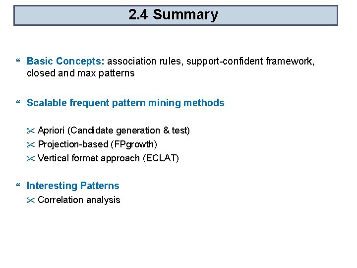
2. 4 Summary Basic Concepts: association rules, support-confident framework, closed and max patterns Scalable frequent pattern mining methods " Apriori (Candidate generation & test) " Projection-based (FPgrowth) " Vertical format approach (ECLAT) Interesting Patterns " Correlation analysis