OLAP and Data Mining Chapter 17 OLTP Compared

OLAP and Data Mining Chapter 17

OLTP Compared With OLAP • On Line Transaction Processing – OLTP – Maintains a database that is an accurate model of some realworld enterprise. Supports day-to-day operations. Characteristics: • Short simple transactions • Relatively frequent updates • Transactions access only a small fraction of the database • On Line Analytic Processing – OLAP – Uses information in database to guide strategic decisions. Characteristics: • • Complex queries Infrequent updates Transactions access a large fraction of the database Data need not be up-to-date 2

The Internet Grocer • OLTP-style transaction: – John Smith, from Schenectady, N. Y. , just bought a box of tomatoes; charge his account; deliver the tomatoes from our Schenectady warehouse; decrease our inventory of tomatoes from that warehouse • OLAP-style transaction: – How many cases of tomatoes were sold in all northeast warehouses in the years 2000 and 2001? 3

OLAP: Traditional Compared with Newer Applications • Traditional OLAP queries – Uses data the enterprise gathers in its usual activities, perhaps in its OLTP system – Queries are ad hoc, perhaps designed and carried out by non-professionals (managers) • Newer Applications (e. g. , Internet companies) – Enterprise actively gathers data it wants, perhaps purchasing it – Queries are sophisticated, designed by professionals, and used in more sophisticated ways 4

The Internet Grocer • Traditional – How many cases of tomatoes were sold in all northeast warehouses in the years 2000 and 2001? • Newer – Prepare a profile of the grocery purchases of John Smith for the years 2000 and 2001 (so that we can customize our marketing to him and get more of his business) 5

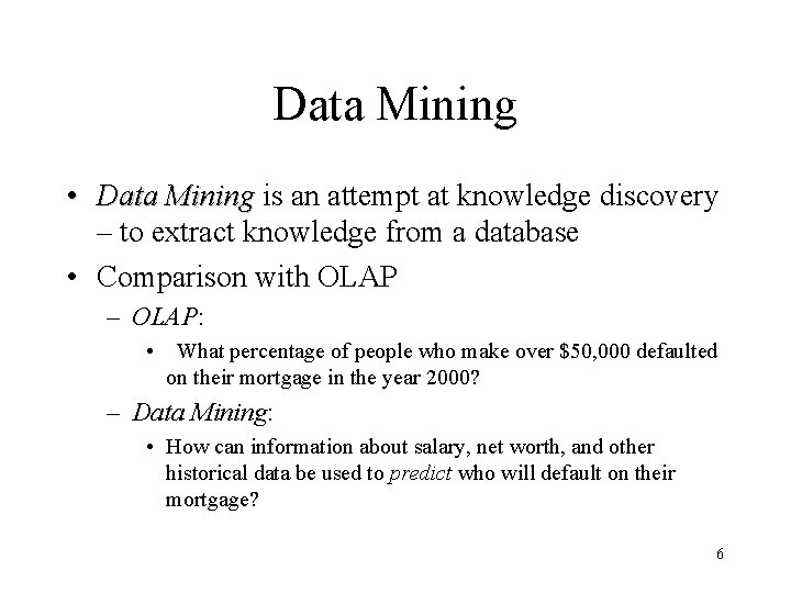
Data Mining • Data Mining is an attempt at knowledge discovery – to extract knowledge from a database • Comparison with OLAP – OLAP: • What percentage of people who make over $50, 000 defaulted on their mortgage in the year 2000? – Data Mining: • How can information about salary, net worth, and other historical data be used to predict who will default on their mortgage? 6

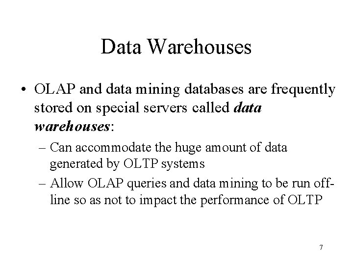
Data Warehouses • OLAP and data mining databases are frequently stored on special servers called data warehouses: – Can accommodate the huge amount of data generated by OLTP systems – Allow OLAP queries and data mining to be run offline so as not to impact the performance of OLTP 7

OLAP, Data Mining, and Analysis • The “A” in OLAP stands for “Analytical” • Many OLAP and Data Mining applications involve sophisticated analysis methods from the fields of mathematics, statistical analysis, and artificial intelligence • Our main interest is in the database aspects of these fields, not the sophisticated analysis techniques 8

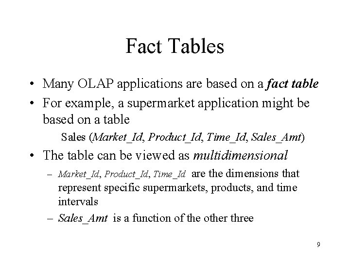
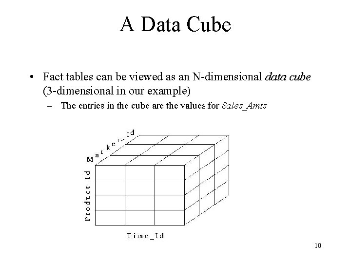
Fact Tables • Many OLAP applications are based on a fact table • For example, a supermarket application might be based on a table Sales (Market_Id, Product_Id, Time_Id, Sales_Amt) • The table can be viewed as multidimensional – Market_Id, Product_Id, Time_Id are the dimensions that represent specific supermarkets, products, and time intervals – Sales_Amt is a function of the other three 9

A Data Cube • Fact tables can be viewed as an N-dimensional data cube (3 -dimensional in our example) – The entries in the cube are the values for Sales_Amts 10

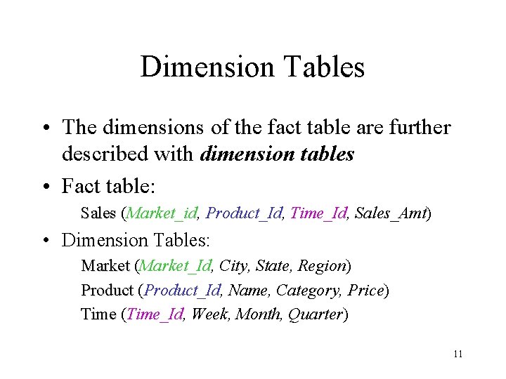
Dimension Tables • The dimensions of the fact table are further described with dimension tables • Fact table: Sales (Market_id, Product_Id, Time_Id, Sales_Amt) • Dimension Tables: Market (Market_Id, City, State, Region) Product (Product_Id, Name, Category, Price) Time (Time_Id, Week, Month, Quarter) 11

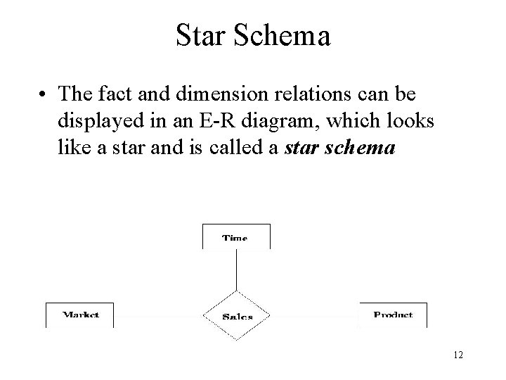
Star Schema • The fact and dimension relations can be displayed in an E-R diagram, which looks like a star and is called a star schema 12

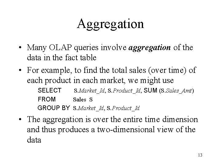
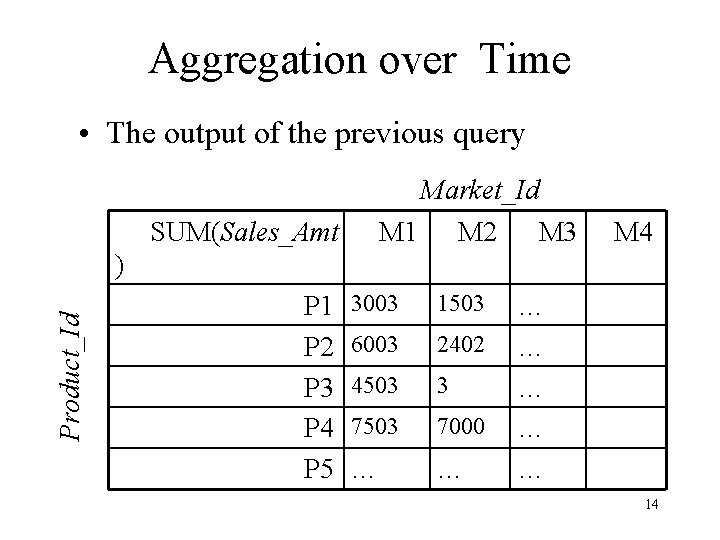
Aggregation • Many OLAP queries involve aggregation of the data in the fact table • For example, to find the total sales (over time) of each product in each market, we might use SELECT S. Market_Id, S. Product_Id, SUM (S. Sales_Amt) FROM Sales S GROUP BY S. Market_Id, S. Product_Id • The aggregation is over the entire time dimension and thus produces a two-dimensional view of the data 13

Aggregation over Time • The output of the previous query Market_Id M 1 M 2 M 3 SUM(Sales_Amt M 4 Product_Id ) P 1 P 2 P 3 P 4 P 5 3003 1503 6003 2402 4503 3 7503 7000 … … … … 14

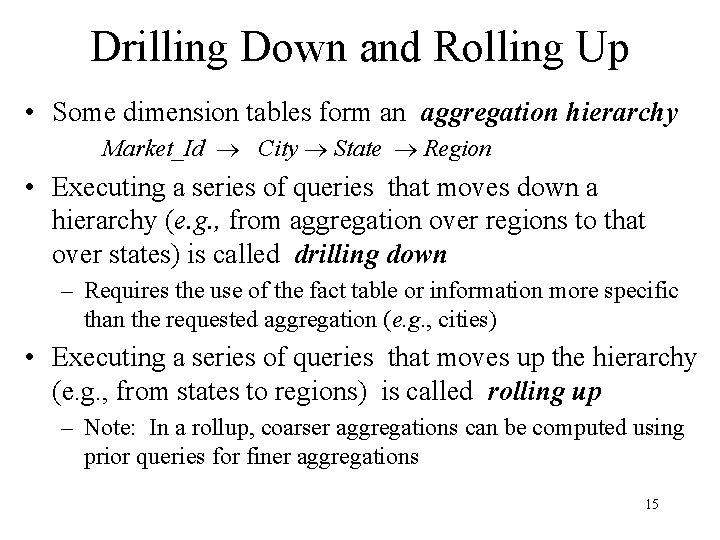
Drilling Down and Rolling Up • Some dimension tables form an aggregation hierarchy Market_Id City State Region • Executing a series of queries that moves down a hierarchy (e. g. , from aggregation over regions to that over states) is called drilling down – Requires the use of the fact table or information more specific than the requested aggregation (e. g. , cities) • Executing a series of queries that moves up the hierarchy (e. g. , from states to regions) is called rolling up – Note: In a rollup, coarser aggregations can be computed using prior queries for finer aggregations 15

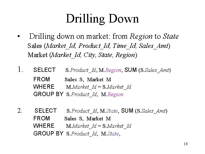
Drilling Down • Drilling down on market: from Region to State Sales (Market_Id, Product_Id, Time_Id, Sales_Amt) Market (Market_Id, City, State, Region) 1. SELECT S. Product_Id, M. Region, SUM (S. Sales_Amt) FROM Sales S, Market M WHERE M. Market_Id = S. Market_Id GROUP BY S. Product_Id, M. Region 2. SELECT S. Product_Id, M. State, SUM (S. Sales_Amt) FROM Sales S, Market M WHERE M. Market_Id = S. Market_Id GROUP BY S. Product_Id, M. State, 16

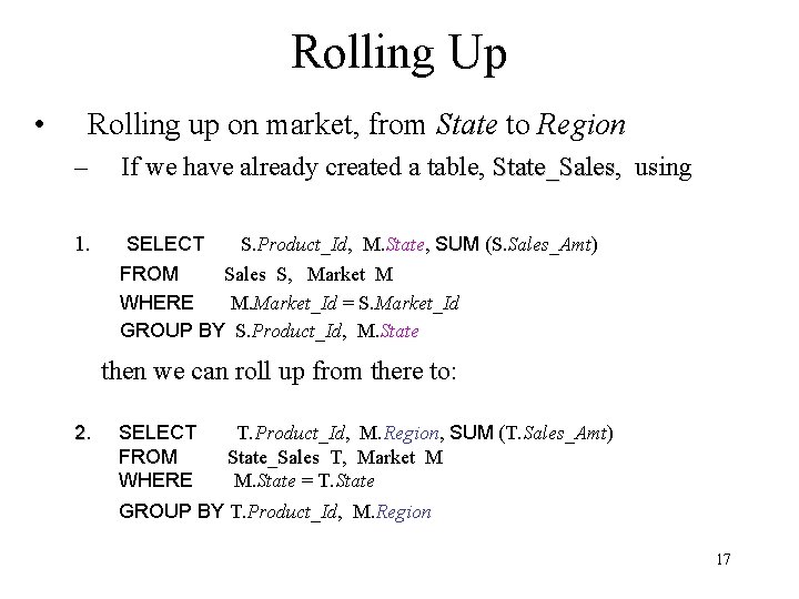
Rolling Up • Rolling up on market, from State to Region – If we have already created a table, State_Sales using 1. SELECT S. Product_Id, M. State, SUM (S. Sales_Amt) FROM Sales S, Market M WHERE M. Market_Id = S. Market_Id GROUP BY S. Product_Id, M. State then we can roll up from there to: 2. SELECT FROM WHERE T. Product_Id, M. Region, SUM (T. Sales_Amt) State_Sales T, Market M M. State = T. State GROUP BY T. Product_Id, M. Region 17

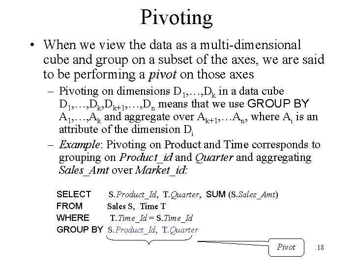
Pivoting • When we view the data as a multi-dimensional cube and group on a subset of the axes, we are said to be performing a pivot on those axes – Pivoting on dimensions D 1, …, Dk in a data cube D 1, …, Dk+1, …, Dn means that we use GROUP BY A 1, …, Ak and aggregate over Ak+1, …An, where Ai is an attribute of the dimension Di – Example: Pivoting on Product and Time corresponds to grouping on Product_id and Quarter and aggregating Sales_Amt over Market_id: SELECT FROM WHERE GROUP BY S. Product_Id, T. Quarter, SUM (S. Sales_Amt) Sales S, Time T T. Time_Id = S. Time_Id S. Product_Id, T. Quarter Pivot 18

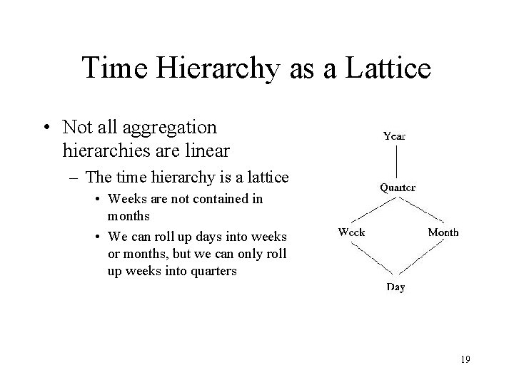
Time Hierarchy as a Lattice • Not all aggregation hierarchies are linear – The time hierarchy is a lattice • Weeks are not contained in months • We can roll up days into weeks or months, but we can only roll up weeks into quarters 19

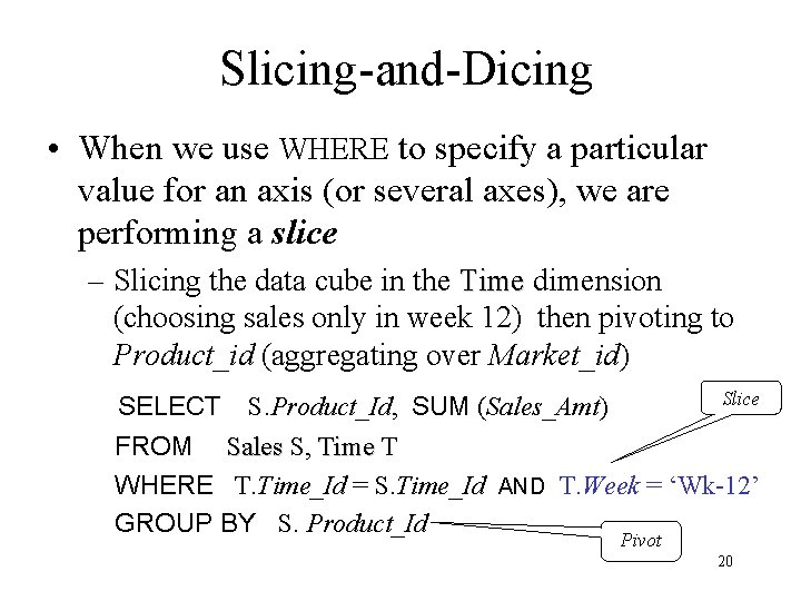
Slicing-and-Dicing • When we use WHERE to specify a particular value for an axis (or several axes), we are performing a slice – Slicing the data cube in the Time dimension (choosing sales only in week 12) then pivoting to Product_id (aggregating over Market_id) SELECT Slice S. Product_Id, SUM (Sales_Amt) FROM Sales S, Time T WHERE T. Time_Id = S. Time_Id AND T. Week = ‘Wk-12’ GROUP BY S. Product_Id Pivot 20

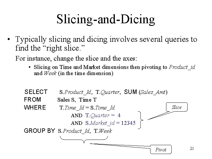
Slicing-and-Dicing • Typically slicing and dicing involves several queries to find the “right slice. ” For instance, change the slice and the axes: • Slicing on Time and Market dimensions then pivoting to Product_id and Week (in the time dimension) SELECT FROM WHERE S. Product_Id, T. Quarter, SUM (Sales_Amt) Sales S, Time T Slice T. Time_Id = S. Time_Id AND T. Quarter = 4 AND S. Market_id = 12345 GROUP BY S. Product_Id, T. Week Pivot 21

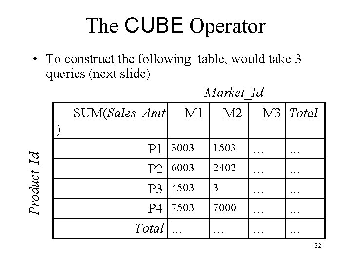
The CUBE Operator Product_Id • To construct the following table, would take 3 queries (next slide) Market_Id SUM(Sales_Amt M 1 M 2 M 3 Total ) P 1 3003 1503 … … P 2 6003 2402 … … P 3 4503 3 … … P 4 7503 7000 … … Total … … 22

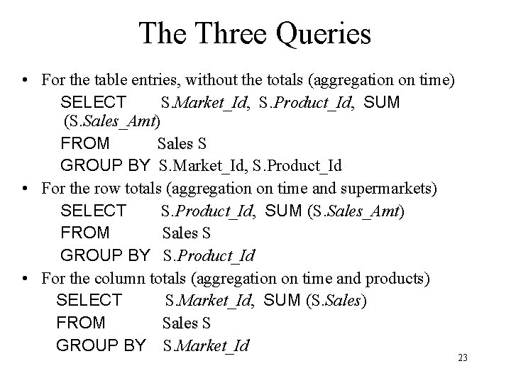
The Three Queries • For the table entries, without the totals (aggregation on time) SELECT S. Market_Id, S. Product_Id, SUM (S. Sales_Amt) FROM Sales S GROUP BY S. Market_Id, S. Product_Id • For the row totals (aggregation on time and supermarkets) SELECT S. Product_Id, SUM (S. Sales_Amt) FROM Sales S GROUP BY S. Product_Id • For the column totals (aggregation on time and products) SELECT S. Market_Id, SUM (S. Sales) FROM Sales S GROUP BY S. Market_Id 23

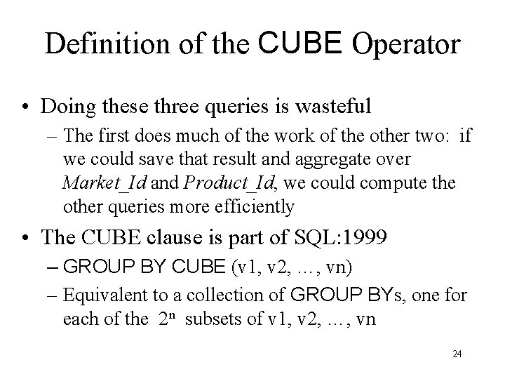
Definition of the CUBE Operator • Doing these three queries is wasteful – The first does much of the work of the other two: if we could save that result and aggregate over Market_Id and Product_Id, we could compute the other queries more efficiently • The CUBE clause is part of SQL: 1999 – GROUP BY CUBE (v 1, v 2, …, vn) – Equivalent to a collection of GROUP BYs, one for each of the 2 n subsets of v 1, v 2, …, vn 24

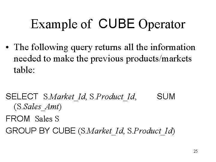
Example of CUBE Operator • The following query returns all the information needed to make the previous products/markets table: SELECT S. Market_Id, S. Product_Id, SUM (S. Sales_Amt) FROM Sales S GROUP BY CUBE (S. Market_Id, S. Product_Id) 25

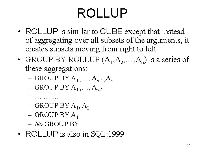
ROLLUP • ROLLUP is similar to CUBE except that instead of aggregating over all subsets of the arguments, it creates subsets moving from right to left • GROUP BY ROLLUP (A 1, A 2, …, An) is a series of these aggregations: – – – GROUP BY A 1 , …, An-1 , An GROUP BY A 1 , …, An-1 ……… GROUP BY A 1, A 2 GROUP BY A 1 No GROUP BY • ROLLUP is also in SQL: 1999 26

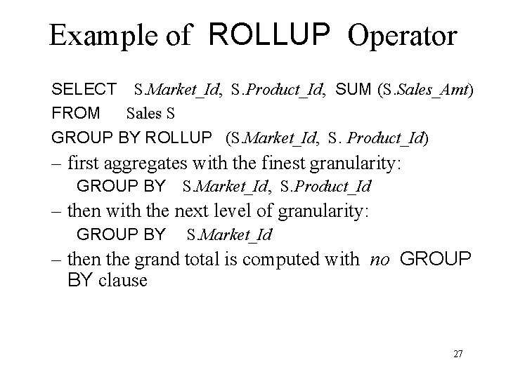
Example of ROLLUP Operator SELECT S. Market_Id, S. Product_Id, SUM (S. Sales_Amt) FROM Sales S GROUP BY ROLLUP (S. Market_Id, S. Product_Id) – first aggregates with the finest granularity: GROUP BY S. Market_Id, S. Product_Id – then with the next level of granularity: GROUP BY S. Market_Id – then the grand total is computed with no GROUP BY clause 27

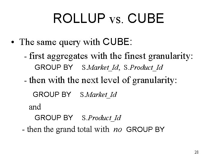
ROLLUP vs. CUBE • The same query with CUBE: - first aggregates with the finest granularity: GROUP BY S. Market_Id, S. Product_Id - then with the next level of granularity: GROUP BY S. Market_Id and GROUP BY S. Product_Id - then the grand total with no GROUP BY 28

Materialized Views The CUBE operator is often used to precompute aggregations on all dimensions of a fact table and then save them as a materialized views to speed up future queries 29

ROLAP and MOLAP • Relational OLAP: ROLAP – OLAP data is stored in a relational database as previously described. Data cube is a conceptual view – way to think about a fact table • Multidimensional OLAP: MOLAP – Vendor provides an OLAP server that implements a fact table as a data cube using a special multi-dimensional (non-relational) data structure 30

MOLAP - No standard query language for MOLAP databases - Many MOLAP vendors (and many ROLAP vendors) provide proprietary visual languages that allow casual users to make queries that involve pivots, drilling down, or rolling up 31

Implementation Issues • OLAP applications are characterized by a very large amount of data that is relatively static, with infrequent updates – Thus, various aggregations can be precomputed and stored in the database – Star joins, join indices, and bitmap indices can be used to improve efficiency (recall the methods to compute star joins in Chapter 14) – Since updates are infrequent, the inefficiencies associated with updates are minimized 32

Data Mining • An attempt at knowledge discovery • Searching for patterns and structure in a sea of data • Uses techniques from many disciplines, such as statistical analysis and machine learning – These techniques are not our main interest 33

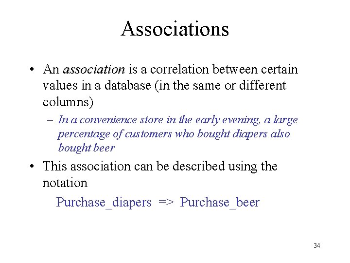
Associations • An association is a correlation between certain values in a database (in the same or different columns) – In a convenience store in the early evening, a large percentage of customers who bought diapers also bought beer • This association can be described using the notation Purchase_diapers => Purchase_beer 34

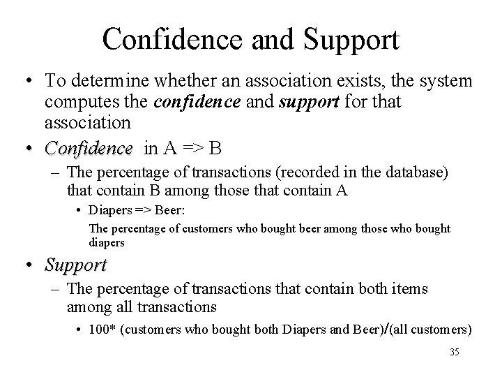
Confidence and Support • To determine whether an association exists, the system computes the confidence and support for that association • Confidence in A => B – The percentage of transactions (recorded in the database) that contain B among those that contain A • Diapers => Beer: The percentage of customers who bought beer among those who bought diapers • Support – The percentage of transactions that contain both items among all transactions • 100* (customers who bought both Diapers and Beer)/(all customers) 35

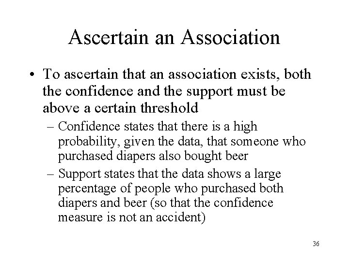
Ascertain an Association • To ascertain that an association exists, both the confidence and the support must be above a certain threshold – Confidence states that there is a high probability, given the data, that someone who purchased diapers also bought beer – Support states that the data shows a large percentage of people who purchased both diapers and beer (so that the confidence measure is not an accident) 36

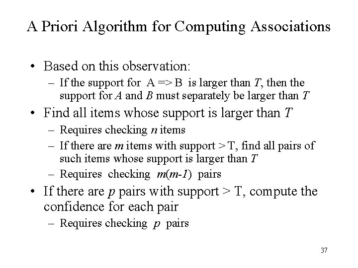
A Priori Algorithm for Computing Associations • Based on this observation: – If the support for A => B is larger than T, then the support for A and B must separately be larger than T • Find all items whose support is larger than T – Requires checking n items – If there are m items with support > T, find all pairs of such items whose support is larger than T – Requires checking m(m-1) pairs • If there are p pairs with support > T, compute the confidence for each pair – Requires checking p pairs 37

Other Types of Information • In addition to association rules, data mining is used to uncover other types of information – Sequential Patterns • Associations over time: Is a customer who purchased a garbage can likely to purchase fillers for that can later? – Classification Rules • Associations based on ranges of values: Can ranges of income be used to classify individuals into groups which predict their likelihood of defaulting on their mortgage? – Time Series • Similarities between sequences: Is the pattern of temperature fluctuation in the Pacific Ocean similar to the pattern of climate variation over the west coast of the US? 38

Another Data Mining Approach • Machine Learning – A mortgage broker believes that several factors might affect whether or not a customer is likely to default on mortgage, but does now know how to weight these factors – Use data from past customers to “learn” a set of weights to be used in the decision for future customers • Neural networks, a technique studied in the context of Artificial Intelligence, provides a model for analyzing this problem 39

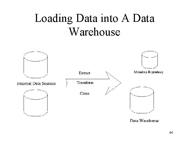
Data Warehouse • Data (often derived from OLTP) for both OLAP and data mining applications is usually stored in a special database called a data warehouse • Data warehouses are generally large and contain data that has been gathered at different times from DBMSs provided by different vendors and with different schemas • Populating such a data warehouse is not trivial 40

Issues Involved in Populating a Data Warehouse • Transformations – Syntactic: syntax used in different DMBSs for the same data might be different • Attribute names: SSN vs. Ssnum • Attribute domains: Integer vs. String – Semantic: semantics might be different • Summarizing sales on a daily basis vs. summarizing sales on a monthly basis • Data Cleaning – Removing errors and inconsistencies in data 41

Metadata • As with other databases, a warehouse must include a metadata repository – Information about physical and logical organization of data – Information about the source of each data item and the dates on which it was loaded and refreshed 42

Incremental Updates • The large volume of data in a data warehouse makes loading and updating a significant task • For efficiency, updating is usually incremental – Different parts are updated at different times • Incremental updates might result in the database being in an inconsistent state – Usually not important because queries involve only statistical summaries of data, which are not greatly affected by such inconsistencies 43

Loading Data into A Data Warehouse 44