Dimensionality Reduction for Data Mining Techniques Applications and

Dimensionality Reduction for Data Mining - Techniques, Applications and Trends Lei Yu Binghamton University Jieping Ye, Huan Liu Arizona State University July 19 -20, 2004

Outline n n Introduction to dimensionality reduction Feature selection (part I) q q n n Basics Representative algorithms Recent advances Applications Feature extraction (part II) Recent trends in dimensionality reduction 2

Why Dimensionality Reduction? n It is so easy and convenient to collect data q n n An experiment Data is not collected only for data mining Data accumulates in an unprecedented speed Data preprocessing is an important part for effective machine learning and data mining Dimensionality reduction is an effective approach to downsizing data 3

Why Dimensionality Reduction? n Most machine learning and data mining techniques may not be effective for highdimensional data q q n Curse of Dimensionality Query accuracy and efficiency degrade rapidly as the dimension increases. The intrinsic dimension may be small. q For example, the number of genes responsible for a certain type of disease may be small. 4

Why Dimensionality Reduction? n Visualization: projection of high-dimensional data onto 2 D or 3 D. n Data compression: efficient storage and retrieval. n Noise removal: positive effect on query accuracy. 5

Application of Dimensionality Reduction n n n n Customer relationship management Text mining Image retrieval Microarray data analysis Protein classification Face recognition Handwritten digit recognition Intrusion detection 6

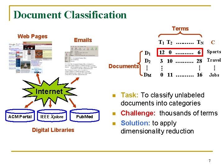
Document Classification Terms C D 1 D 2 12 0 …. …… 6 Sports Internet ACM Portal IEEE Xplore n Pub. Med n n Digital Libraries 0 11 …. …… 16 … DM 3 10 …. …… 28 Travel … Documents T 1 T 2 …. …… TN … Emails … Web Pages Jobs Task: To classify unlabeled documents into categories Challenge: thousands of terms Solution: to apply dimensionality reduction 7

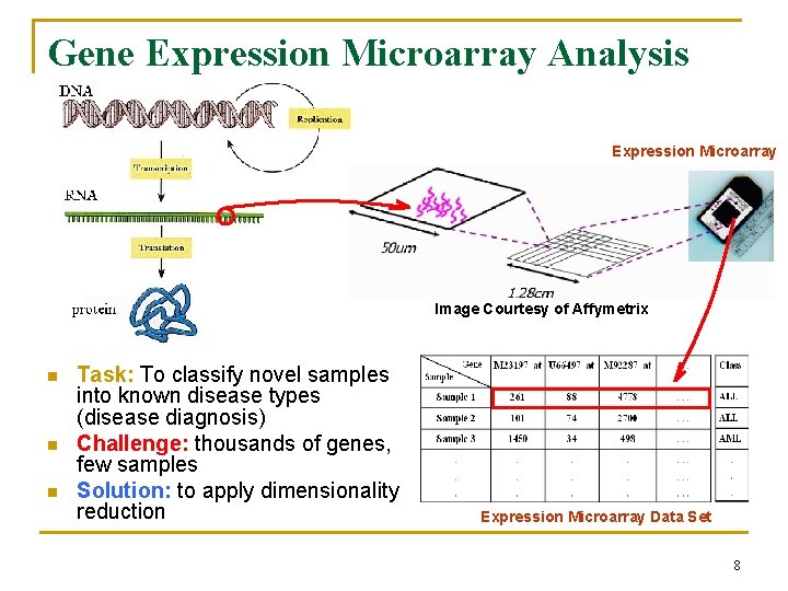
Gene Expression Microarray Analysis Expression Microarray Image Courtesy of Affymetrix n n n Task: To classify novel samples into known disease types (disease diagnosis) Challenge: thousands of genes, few samples Solution: to apply dimensionality reduction Expression Microarray Data Set 8

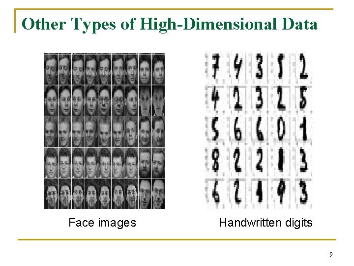
Other Types of High-Dimensional Data Face images Handwritten digits 9

Major Techniques of Dimensionality Reduction n Feature selection q q n Feature Extraction (reduction) q q n Definition Objectives Differences between the two techniques 10

Feature Selection n Definition q n A process that chooses an optimal subset of features according to a objective function Objectives q q To reduce dimensionality and remove noise To improve mining performance n n n Speed of learning Predictive accuracy Simplicity and comprehensibility of mined results 11

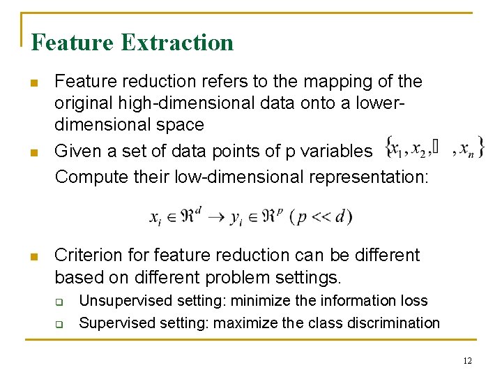
Feature Extraction Feature reduction refers to the mapping of the original high-dimensional data onto a lowerdimensional space n Given a set of data points of p variables Compute their low-dimensional representation: n n Criterion for feature reduction can be different based on different problem settings. q q Unsupervised setting: minimize the information loss Supervised setting: maximize the class discrimination 12

Feature Reduction vs. Feature Selection n Feature reduction q q n Feature selection q n All original features are used The transformed features are linear combinations of the original features Only a subset of the original features are selected Continuous versus discrete 13

Outline n n Introduction to dimensionality reduction Feature selection (part I) q q n n Basics Representative algorithms Recent advances Applications Feature extraction (part II) Recent trends in dimensionality reduction 14

Basics n n Definitions of subset optimality Perspectives of feature selection q q Subset search and feature ranking Feature/subset evaluation measures Models: filter vs. wrapper Results validation and evaluation 15

Subset Optimality for Classification n A minimum subset that is sufficient to construct a hypothesis consistent with the training examples (Almuallim and Dietterich, AAAI, 1991) q q n Optimality is based on training set The optimal set may overfit the training data A minimum subset G such that P(C|G) is equal or as close as possible to P(C|F) (Koller and Sahami, ICML, 1996) q q Optimality is based on the entire population Only training part of the data is available 16

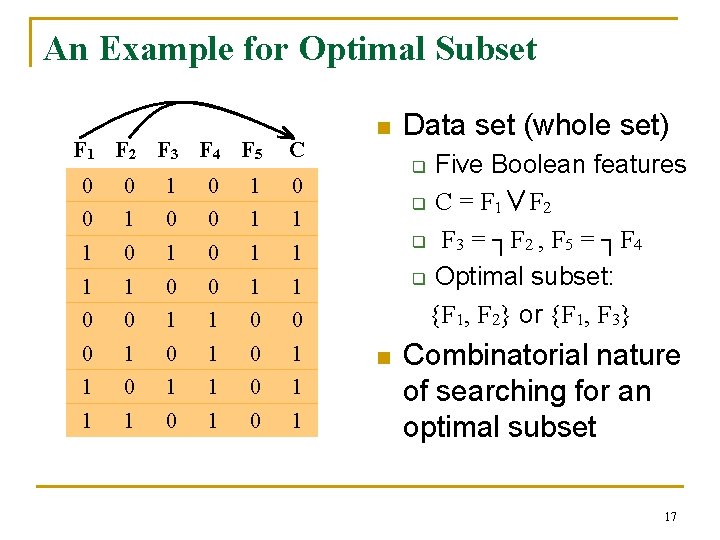
An Example for Optimal Subset F 1 F 2 F 3 F 4 F 5 C 0 0 1 1 1 0 0 1 1 0 0 0 1 0 1 1 1 0 1 n Data set (whole set) Five Boolean features q C = F 1∨F 2 q F 3 = ┐F 2 , F 5 = ┐F 4 q Optimal subset: {F 1, F 2} or {F 1, F 3} q n Combinatorial nature of searching for an optimal subset 17

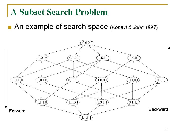
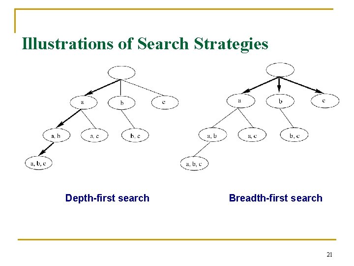
A Subset Search Problem n An example of search space (Kohavi & John 1997) Forward Backward 18

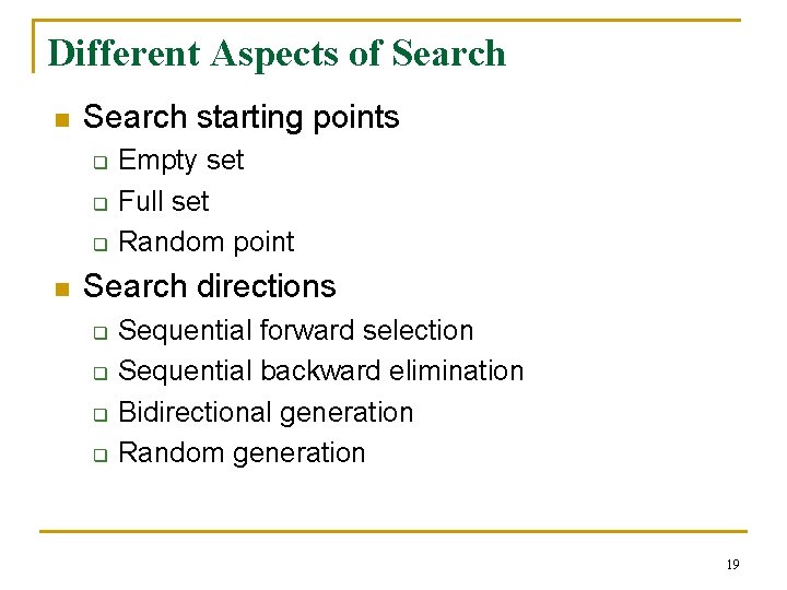
Different Aspects of Search n Search starting points q q q n Empty set Full set Random point Search directions q q Sequential forward selection Sequential backward elimination Bidirectional generation Random generation 19

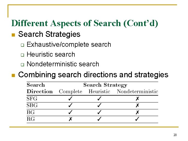
Different Aspects of Search (Cont’d) n Search Strategies q q q n Exhaustive/complete search Heuristic search Nondeterministic search Combining search directions and strategies 20

Illustrations of Search Strategies Depth-first search Breadth-first search 21

Feature Ranking n n n Weighting and ranking individual features Selecting top-ranked ones for feature selection Advantages q q n Efficient: O(N) in terms of dimensionality N Easy to implement Disadvantages q q Hard to determine threshold Unable to consider correlation between features 22

Evaluation Measures for Ranking and Selecting Features n n The goodness of a feature/feature subset is dependent on measures Various measures Information measures (Yu & Liu 2004, Jebara & Jaakkola 2000) q Distance measures (Robnik & Kononenko 03, Pudil & Novovicov 98) q Dependence measures (Hall 2000, Modrzejewski 1993) q Consistency measures (Almuallim & Dietterich 94, Dash & Liu 03) q Accuracy measures (Dash & Liu 2000, Kohavi&John 1997) q 23

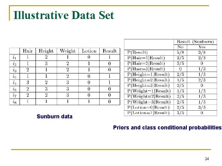
Illustrative Data Set Sunburn data Priors and class conditional probabilities 24

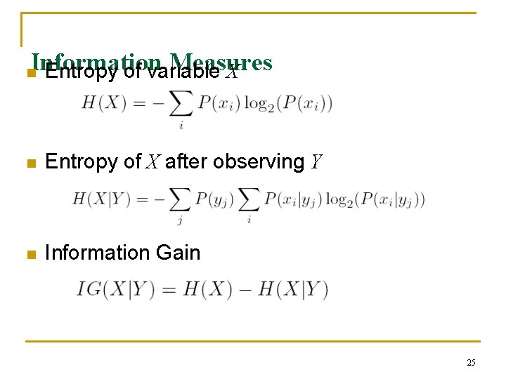
Information Measures Entropy of variable X n n Entropy of X after observing Y n Information Gain 25

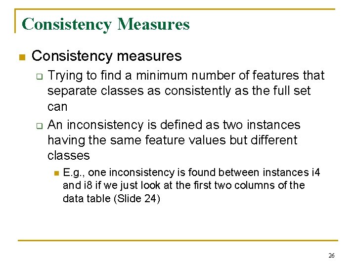
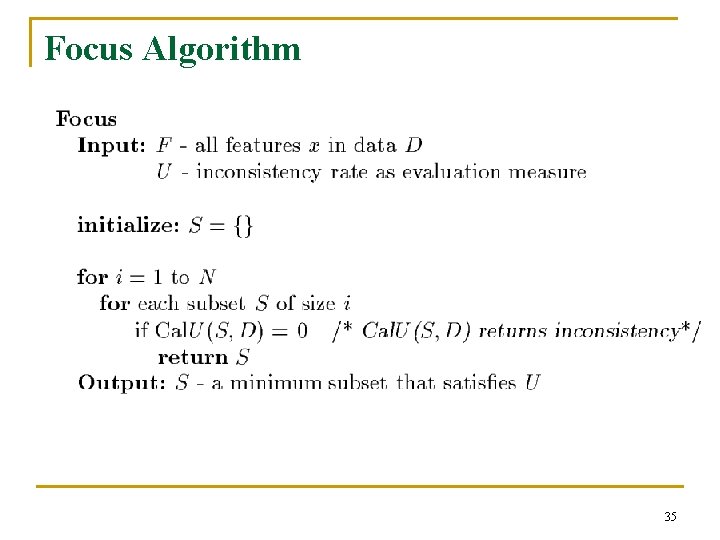
Consistency Measures n Consistency measures q q Trying to find a minimum number of features that separate classes as consistently as the full set can An inconsistency is defined as two instances having the same feature values but different classes n E. g. , one inconsistency is found between instances i 4 and i 8 if we just look at the first two columns of the data table (Slide 24) 26

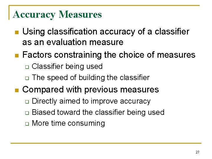
Accuracy Measures n n Using classification accuracy of a classifier as an evaluation measure Factors constraining the choice of measures q q n Classifier being used The speed of building the classifier Compared with previous measures q q q Directly aimed to improve accuracy Biased toward the classifier being used More time consuming 27

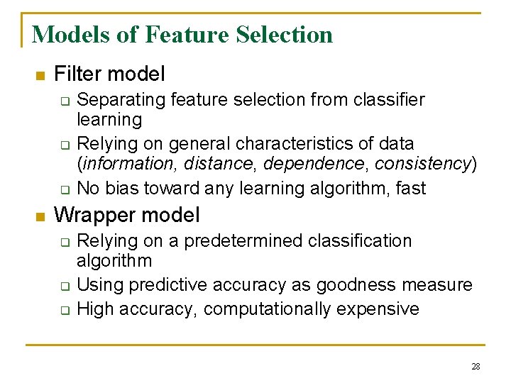
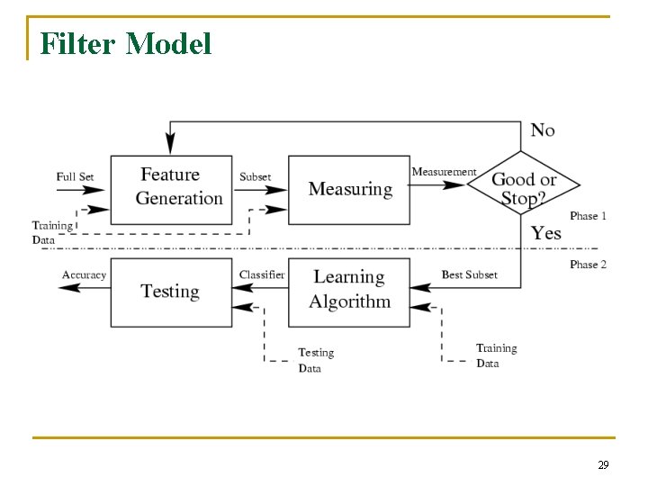
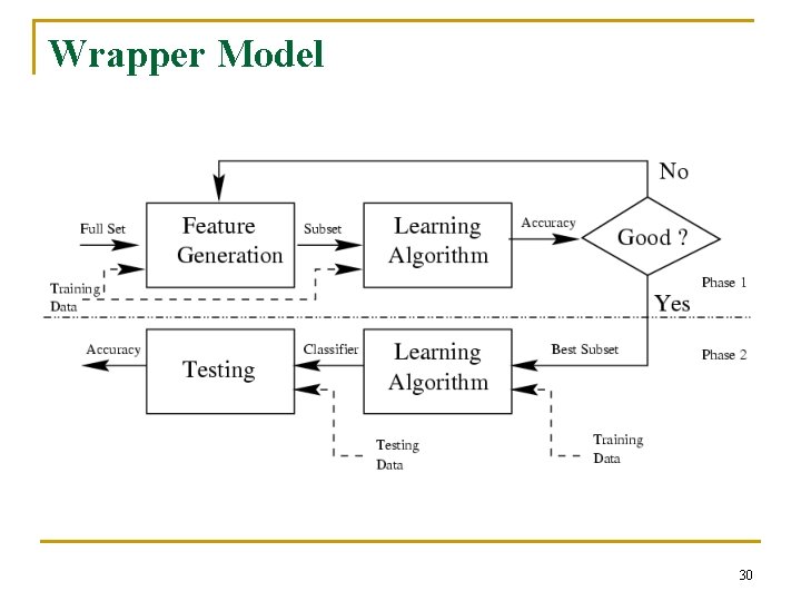
Models of Feature Selection n Filter model q q q n Separating feature selection from classifier learning Relying on general characteristics of data (information, distance, dependence, consistency) No bias toward any learning algorithm, fast Wrapper model q q q Relying on a predetermined classification algorithm Using predictive accuracy as goodness measure High accuracy, computationally expensive 28

Filter Model 29

Wrapper Model 30

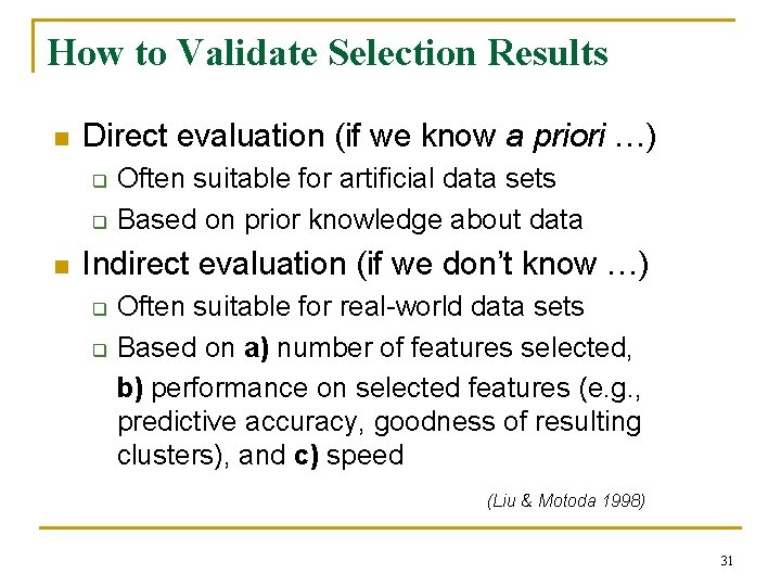
How to Validate Selection Results n Direct evaluation (if we know a priori …) q q n Often suitable for artificial data sets Based on prior knowledge about data Indirect evaluation (if we don’t know …) Often suitable for real-world data sets q Based on a) number of features selected, b) performance on selected features (e. g. , predictive accuracy, goodness of resulting clusters), and c) speed q (Liu & Motoda 1998) 31

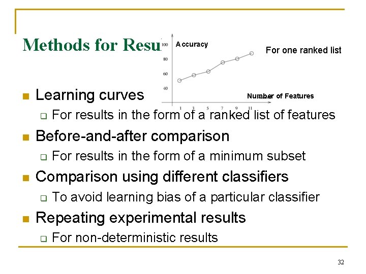
Methods for Result Evaluation For one ranked list Accuracy n Learning curves q n For results in the form of a minimum subset Comparison using different classifiers q n For results in the form of a ranked list of features Before-and-after comparison q n Number of Features To avoid learning bias of a particular classifier Repeating experimental results q For non-deterministic results 32

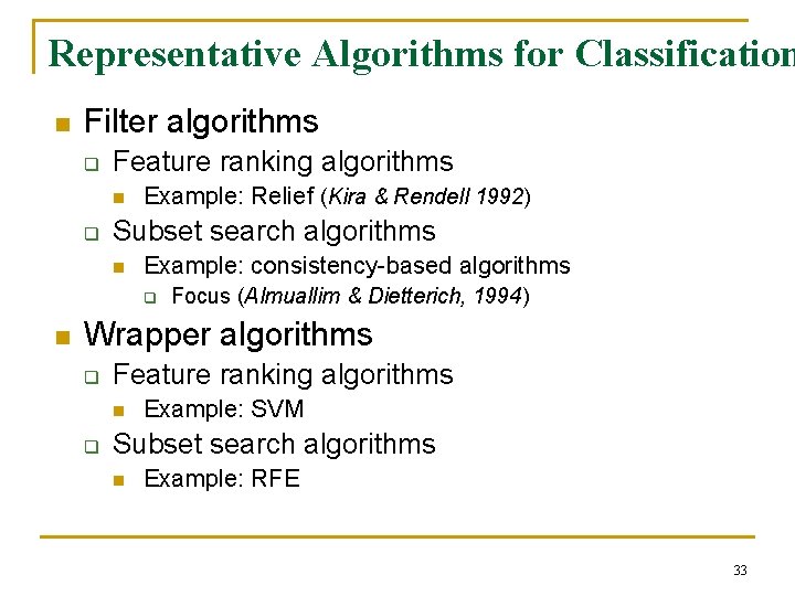
Representative Algorithms for Classification n Filter algorithms q Feature ranking algorithms n q Example: Relief (Kira & Rendell 1992) Subset search algorithms n Example: consistency-based algorithms q n Focus (Almuallim & Dietterich, 1994) Wrapper algorithms q Feature ranking algorithms n q Example: SVM Subset search algorithms n Example: RFE 33

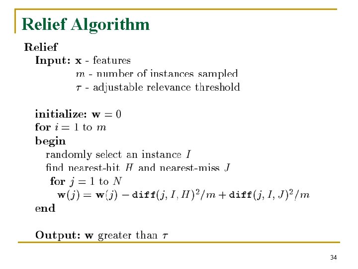
Relief Algorithm 34

Focus Algorithm 35

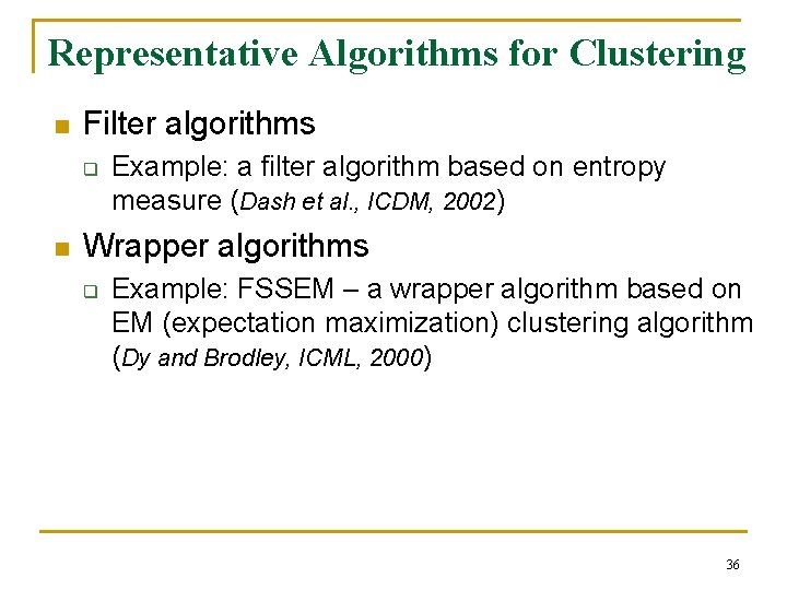
Representative Algorithms for Clustering n Filter algorithms q n Example: a filter algorithm based on entropy measure (Dash et al. , ICDM, 2002) Wrapper algorithms q Example: FSSEM – a wrapper algorithm based on EM (expectation maximization) clustering algorithm (Dy and Brodley, ICML, 2000) 36

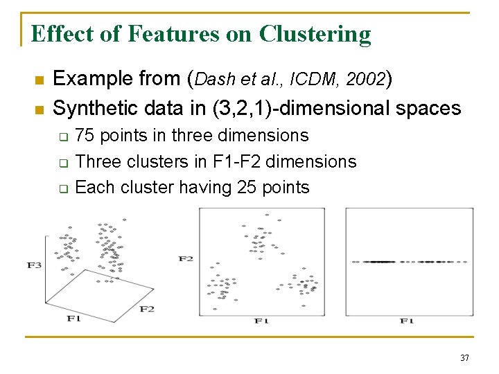
Effect of Features on Clustering n n Example from (Dash et al. , ICDM, 2002) Synthetic data in (3, 2, 1)-dimensional spaces q q q 75 points in three dimensions Three clusters in F 1 -F 2 dimensions Each cluster having 25 points 37

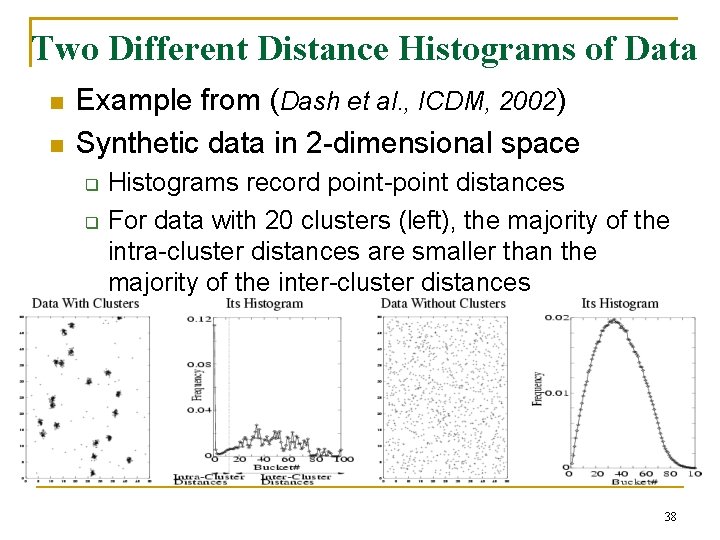
Two Different Distance Histograms of Data n n Example from (Dash et al. , ICDM, 2002) Synthetic data in 2 -dimensional space q q Histograms record point-point distances For data with 20 clusters (left), the majority of the intra-cluster distances are smaller than the majority of the inter-cluster distances 38

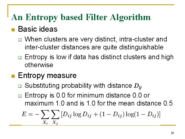
An Entropy based Filter Algorithm n Basic ideas q q n When clusters are very distinct, intra-cluster and inter-cluster distances are quite distinguishable Entropy is low if data has distinct clusters and high otherwise Entropy measure q q Substituting probability with distance Dij Entropy is 0. 0 for minimum distance 0. 0 or maximum 1. 0 and is 1. 0 for the mean distance 0. 5 39

FSSEM Algorithm n EM Clustering q q n To estimate the maximum likelihood mixture model parameters and the cluster probabilities of each data point Each data point belongs to every cluster with some probability Feature selection for EM q q q Searching through feature subsets Applying EM on each candidate subset Evaluating goodness of each candidate subset based on the goodness of resulting clusters 40

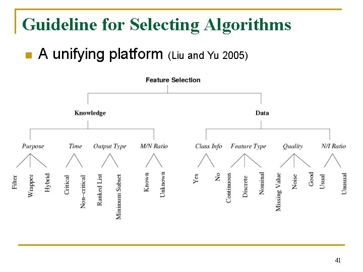
Guideline for Selecting Algorithms n A unifying platform (Liu and Yu 2005) 41

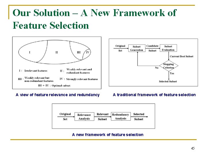
Handling High-dimensional Data n High-dimensional data q q q n As in gene expression microarray analysis, text categorization, … With hundreds to tens of thousands of features With many irrelevant and redundant features Recent research results q Redundancy based feature selection n Yu and Liu, ICML-2003, JMLR-2004 42

Limitations of Existing Methods n Individual feature evaluation q q n Focusing on identifying relevant features without handling feature redundancy Time complexity: O(N) Feature subset evaluation q q Relying on minimum feature subset heuristics to implicitly handling redundancy while pursuing relevant features Time complexity: at least O(N 2) 43

Goals n High effectiveness q q n Able to handle both irrelevant and redundant features Not pure individual feature evaluation High efficiency q q Less costly than existing subset evaluation methods Not traditional heuristic search methods 44

Our Solution – A New Framework of Feature Selection A view of feature relevance and redundancy A traditional framework of feature selection A new framework of feature selection 45

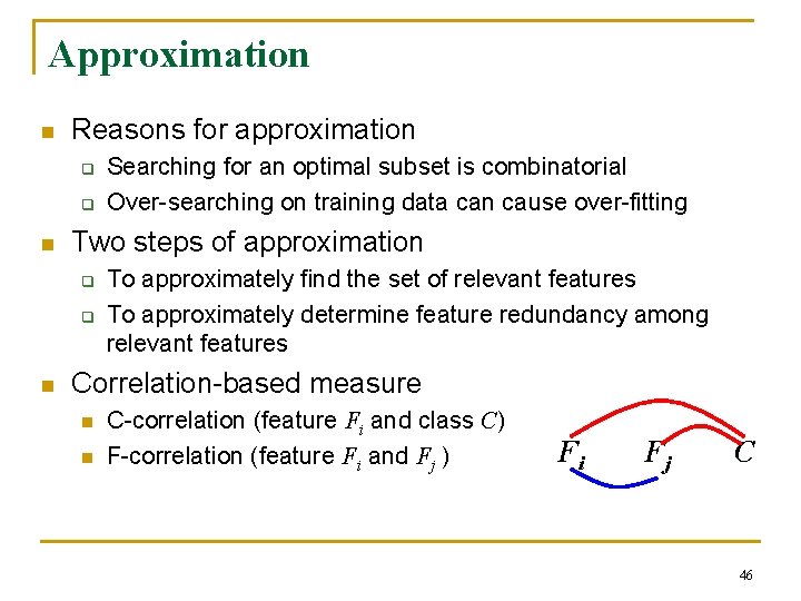
Approximation n Reasons for approximation q q n Two steps of approximation q q n Searching for an optimal subset is combinatorial Over-searching on training data can cause over-fitting To approximately find the set of relevant features To approximately determine feature redundancy among relevant features Correlation-based measure n n C-correlation (feature Fi and class C) F-correlation (feature Fi and Fj ) Fi Fj C 46

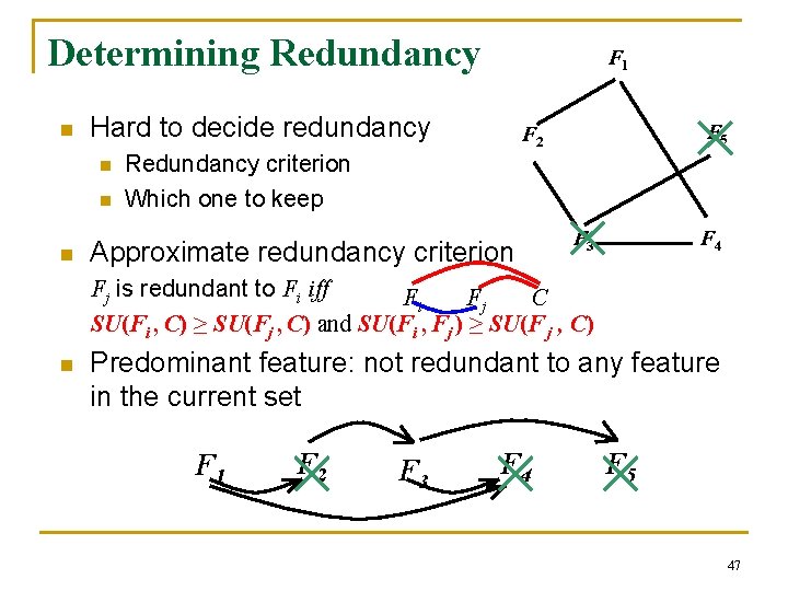
Determining Redundancy n Hard to decide redundancy n n n F 1 F 5 F 2 Redundancy criterion Which one to keep Approximate redundancy criterion F 3 F 4 Fj is redundant to Fi iff Fi Fj C SU(Fi , C) ≥ SU(Fj , C) and SU(Fi , Fj ) ≥ SU(F j , C) n Predominant feature: not redundant to any feature in the current set F 1 F 2 F 3 F 4 F 5 47

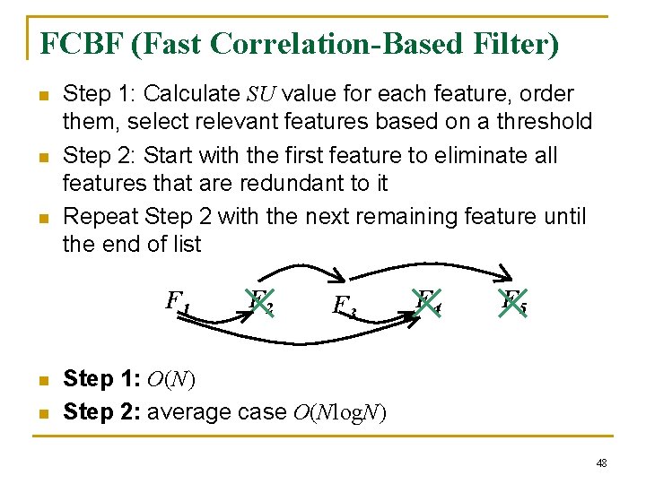
FCBF (Fast Correlation-Based Filter) n n n Step 1: Calculate SU value for each feature, order them, select relevant features based on a threshold Step 2: Start with the first feature to eliminate all features that are redundant to it Repeat Step 2 with the next remaining feature until the end of list F 1 n n F 2 F 3 F 4 F 5 Step 1: O(N) Step 2: average case O(Nlog. N) 48

Real-World Applications n Customer relationship management q n Text categorization q q n q Swets and Weng, 1995 (MSU) Dy et al. , 2003 (Purdue University) Gene expression microarrray data analysis q q n Yang and Pederson, 1997 (CMU) Forman, 2003 (HP Labs) Image retrieval q n Ng and Liu, 2000 (NUS) Golub et al. , 1999 (MIT) Xing et al. , 2001 (UC Berkeley) Intrusion detection q Lee et al. , 2000 (Columbia University) 49

Text Categorization n Text categorization q q n Difficulty from high-dimensionality q q n Automatically assigning predefined categories to new text documents Of great importance given massive on-line text from WWW, Emails, digital libraries… Each unique term (word or phrase) representing a feature in the original feature space Hundreds or thousands of unique terms for even a moderate-sized text collection Desirable to reduce the feature space without sacrificing categorization accuracy 50

Feature Selection in Text Categorization n A comparative study in (Yang and Pederson, ICML, 1997) q q n 5 metrics evaluated and compared n Document Frequency (DF), Information Gain (IG), Mutual Information (MU), X 2 statistics (CHI), Term Strength (TS) n IG and CHI performed the best Improved classification accuracy of k-NN achieved after removal of up to 98% unique terms by IG Another study in (Forman, JMLR, 2003) q q 12 metrics evaluated on 229 categorization problems A new metric, Bi-Normal Separation, outperformed others and improved accuracy of SVMs 51

Content-Based Image Retrieval (CBIR) n Image retrieval q q n Content-based image retrieval (CBIR) q q n An explosion of image collections from scientific, civil, military equipments Necessary to index the images for efficient retrieval Instead of indexing images based on textual descriptions (e. g. , keywords, captions) Indexing images based on visual contents (e. g. , color, texture, shape) Traditional methods for CBIR q q Using all indexes (features) to compare images Hard to scale to large size image collections 52

Feature Selection in CBIR n An application in (Swets and Weng, ISCV, 1995) q q n A large database of widely varying real-world objects in natural settings Selecting relevant features to index images for efficient retrieval Another application in (Dy et al. , Trans. PRMI, 2003) q q q A database of high resolution computed tomography lung images FSSEM algorithm applied to select critical characterizing features Retrieval precision improved based on selected features 53

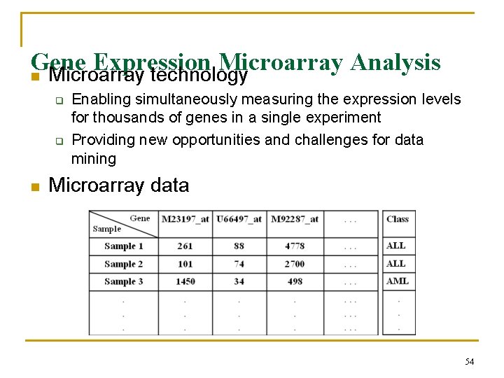
Gene Expression Microarray Analysis n Microarray technology q q n Enabling simultaneously measuring the expression levels for thousands of genes in a single experiment Providing new opportunities and challenges for data mining Microarray data 54

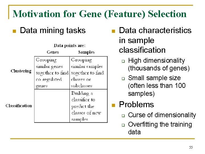
Motivation for Gene (Feature) Selection n Data mining tasks n Data characteristics in sample classification q q n High dimensionality (thousands of genes) Small sample size (often less than 100 samples) Problems q q Curse of dimensionality Overfitting the training data 55

Feature Selection in Sample Classification n An application in (Golub, Science, 1999) q q q n On leukemia data (7129 genes, 72 samples) Feature ranking method based on linear correlation Classification accuracy improved by 50 top genes Another application in (Xing et al. , ICML, 2001) q A hybrid of filter and wrapper method n n q Selecting best subset of each cardinality based on information gain ranking and Markov blanket filtering Comparing between subsets of the same cardinality using cross-validation Accuracy improvements observed on the same leukemia data 56

Intrusion Detection via Data Mining n Network-based computer systems q q n n Playing increasingly vital roles in modern society Targets of attacks from enemies and criminals Intrusion detection is one way to protect computer systems A data mining framework for intrusion detection in (Lee et al. , AI Review, 2000) q q Audit data analyzed using data mining algorithms to obtain frequent activity patterns Classifiers based on selected features used to classify an observed system activity as “legitimate” or “intrusive” 57

Dimensionality Reduction for Data Mining - Techniques, Applications and Trends (Part II) Lei Yu Binghamton University Jieping Ye, Huan Liu Arizona State University July 19 -20, 2004

Outline n n n Introduction to dimensionality reduction Feature selection (part I) Feature extraction (part II) q q n Basics Representative algorithms Recent advances Applications Recent trends in dimensionality reduction 59

Feature Reduction Algorithms n Unsupervised q q n Supervised q q q n Latent Semantic Indexing (LSI): truncated SVD Independent Component Analysis (ICA) Principal Component Analysis (PCA) Manifold learning algorithms Linear Discriminant Analysis (LDA) Canonical Correlation Analysis (CCA) Partial Least Squares (PLS) Semi-supervised 60

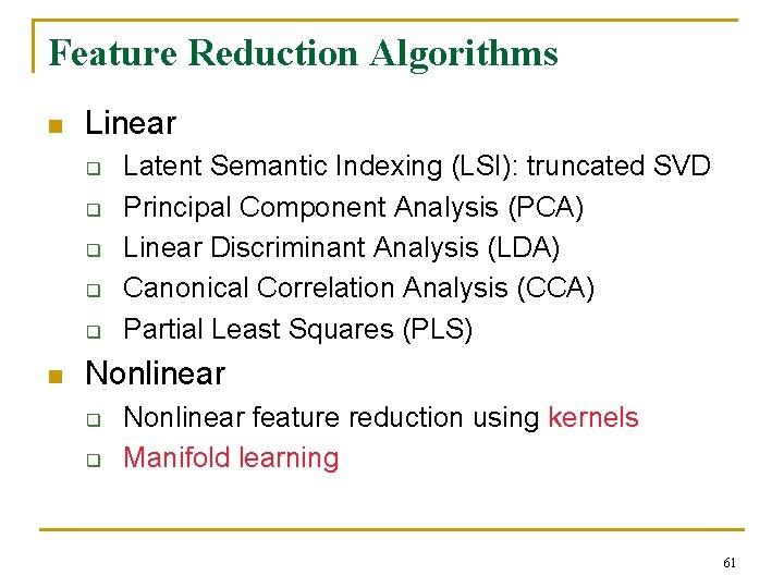
Feature Reduction Algorithms n Linear q q q n Latent Semantic Indexing (LSI): truncated SVD Principal Component Analysis (PCA) Linear Discriminant Analysis (LDA) Canonical Correlation Analysis (CCA) Partial Least Squares (PLS) Nonlinear q q Nonlinear feature reduction using kernels Manifold learning 61

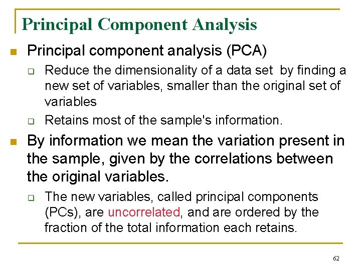
Principal Component Analysis n Principal component analysis (PCA) q q n Reduce the dimensionality of a data set by finding a new set of variables, smaller than the original set of variables Retains most of the sample's information. By information we mean the variation present in the sample, given by the correlations between the original variables. q The new variables, called principal components (PCs), are uncorrelated, and are ordered by the fraction of the total information each retains. 62

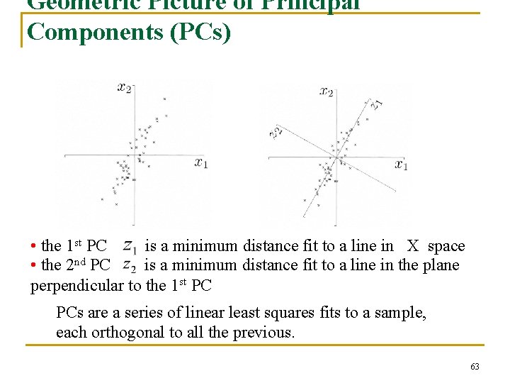
Geometric Picture of Principal Components (PCs) • the 1 st PC is a minimum distance fit to a line in X space • the 2 nd PC is a minimum distance fit to a line in the plane perpendicular to the 1 st PC PCs are a series of linear least squares fits to a sample, each orthogonal to all the previous. 63

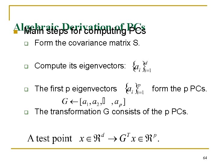
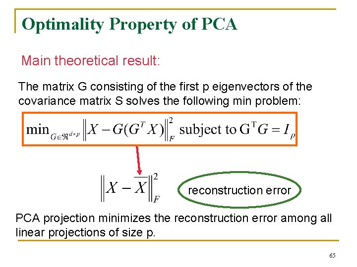
Algebraic Derivation of PCs n Main steps for computing PCs q Form the covariance matrix S. q Compute its eigenvectors: q The first p eigenvectors form the p PCs. q The transformation G consists of the p PCs. 64

Optimality Property of PCA Main theoretical result: The matrix G consisting of the first p eigenvectors of the covariance matrix S solves the following min problem: reconstruction error PCA projection minimizes the reconstruction error among all linear projections of size p. 65

Applications of PCA n n n Eigenfaces for recognition. Turk and Pentland. 1991. Principal Component Analysis for clustering gene expression data. Yeung and Ruzzo. 2001. Probabilistic Disease Classification of Expression-Dependent Proteomic Data from Mass Spectrometry of Human Serum. Lilien. 2003. 66

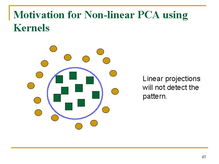
Motivation for Non-linear PCA using Kernels Linear projections will not detect the pattern. 67

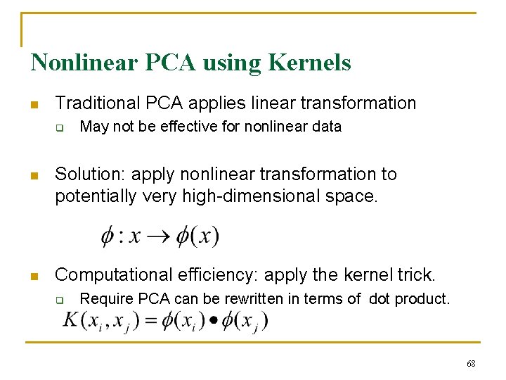
Nonlinear PCA using Kernels n Traditional PCA applies linear transformation q May not be effective for nonlinear data n Solution: apply nonlinear transformation to potentially very high-dimensional space. n Computational efficiency: apply the kernel trick. q Require PCA can be rewritten in terms of dot product. 68

Canonical Correlation Analysis (CCA) n CCA was developed first by H. Hotelling. q n n n H. Hotelling. Relations between two sets of variates. Biometrika, 28: 321 -377, 1936. CCA measures the linear relationship between two multidimensional variables. CCA finds two bases, one for each variable, that are optimal with respect to correlations. Applications in economics, medical studies, bioinformatics and other areas. 69

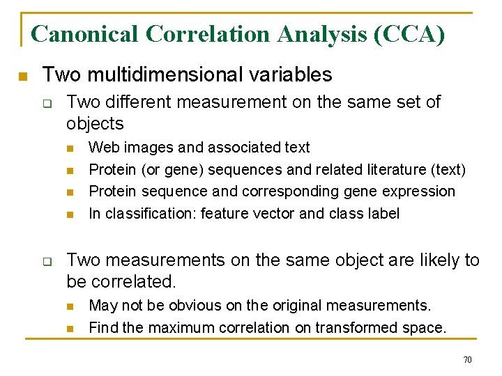
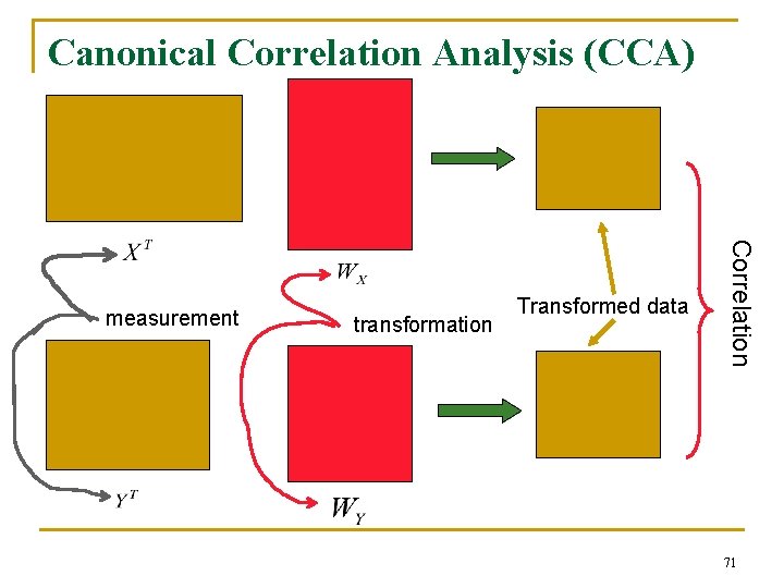
Canonical Correlation Analysis (CCA) n Two multidimensional variables q Two different measurement on the same set of objects n n q Web images and associated text Protein (or gene) sequences and related literature (text) Protein sequence and corresponding gene expression In classification: feature vector and class label Two measurements on the same object are likely to be correlated. n n May not be obvious on the original measurements. Find the maximum correlation on transformed space. 70

Canonical Correlation Analysis (CCA) transformation Transformed data Correlation measurement 71

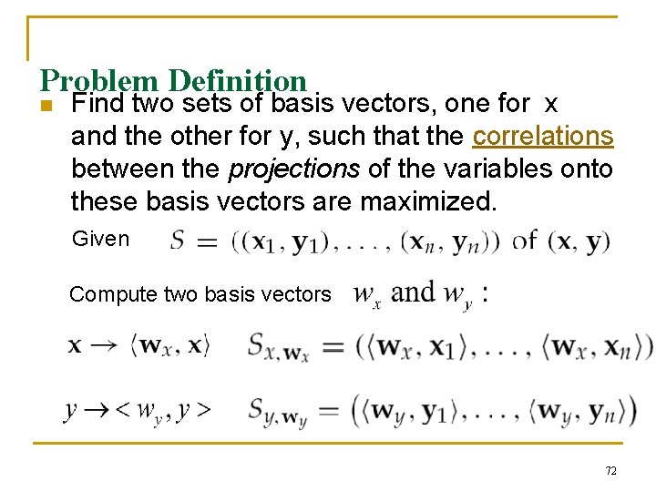
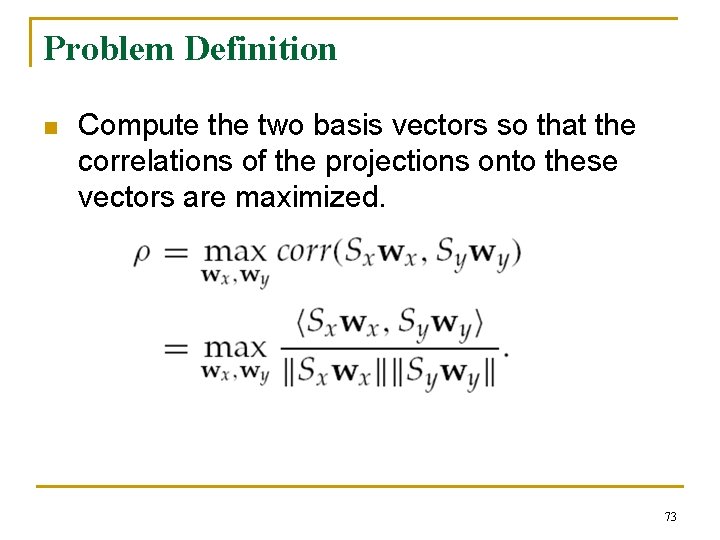
Problem Definition n Find two sets of basis vectors, one for x and the other for y, such that the correlations between the projections of the variables onto these basis vectors are maximized. Given Compute two basis vectors 72

Problem Definition n Compute the two basis vectors so that the correlations of the projections onto these vectors are maximized. 73

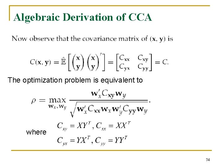
Algebraic Derivation of CCA The optimization problem is equivalent to where 74

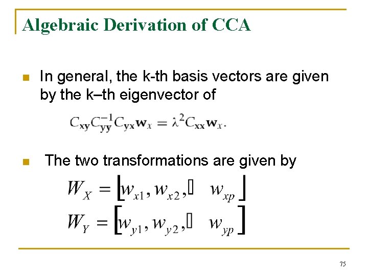
Algebraic Derivation of CCA n In general, the k-th basis vectors are given by the k–th eigenvector of n The two transformations are given by 75

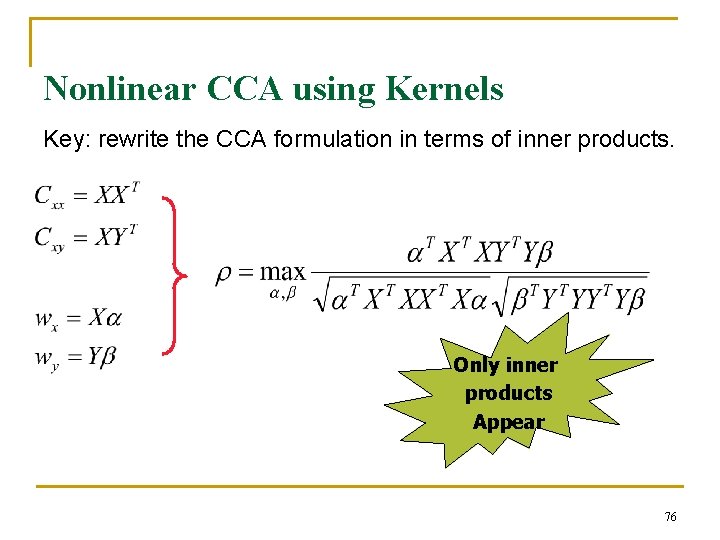
Nonlinear CCA using Kernels Key: rewrite the CCA formulation in terms of inner products. Only inner products Appear 76

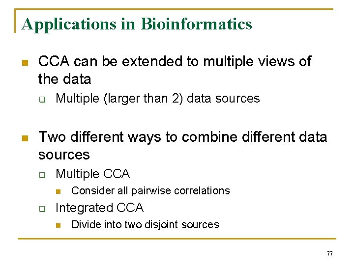
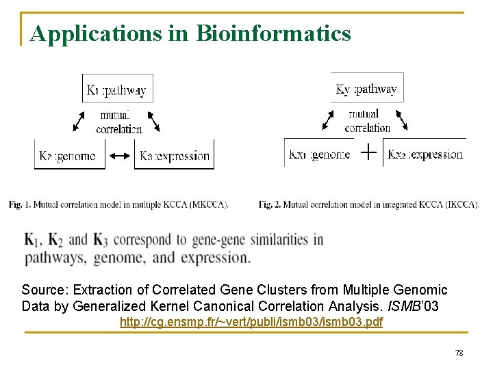
Applications in Bioinformatics n CCA can be extended to multiple views of the data q n Multiple (larger than 2) data sources Two different ways to combine different data sources q Multiple CCA n q Consider all pairwise correlations Integrated CCA n Divide into two disjoint sources 77

Applications in Bioinformatics Source: Extraction of Correlated Gene Clusters from Multiple Genomic Data by Generalized Kernel Canonical Correlation Analysis. ISMB’ 03 http: //cg. ensmp. fr/~vert/publi/ismb 03. pdf 78

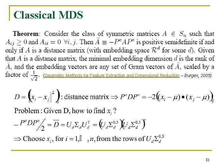
Multidimensional scaling (MDS) • MDS: Multidimensional scaling • Borg and Groenen, 1997 • MDS takes a matrix of pair-wise distances and gives a mapping to Rd. It finds an embedding that preserves the interpoint distances, equivalent to PCA when those distance are Euclidean. • Low dimensional data for visualization 79

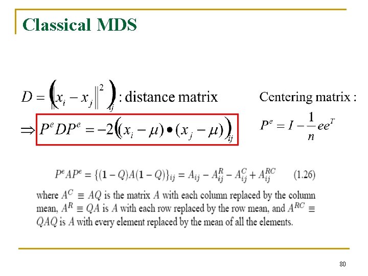
Classical MDS 80

Classical MDS (Geometric Methods for Feature Extraction and Dimensional Reduction – Burges, 2005) 81

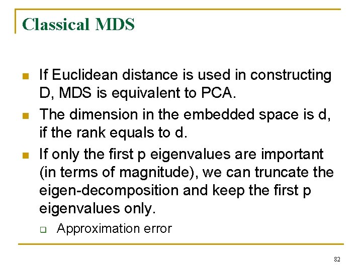
Classical MDS n n n If Euclidean distance is used in constructing D, MDS is equivalent to PCA. The dimension in the embedded space is d, if the rank equals to d. If only the first p eigenvalues are important (in terms of magnitude), we can truncate the eigen-decomposition and keep the first p eigenvalues only. q Approximation error 82

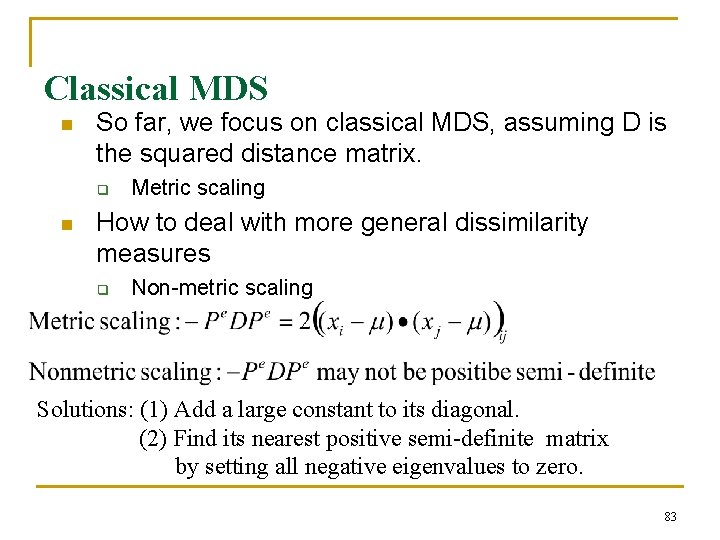
Classical MDS n So far, we focus on classical MDS, assuming D is the squared distance matrix. q n Metric scaling How to deal with more general dissimilarity measures q Non-metric scaling Solutions: (1) Add a large constant to its diagonal. (2) Find its nearest positive semi-definite matrix by setting all negative eigenvalues to zero. 83

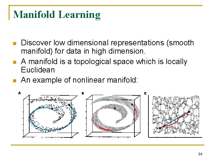
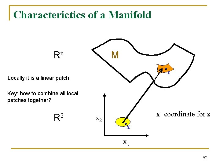
Manifold Learning n n n Discover low dimensional representations (smooth manifold) for data in high dimension. A manifold is a topological space which is locally Euclidean An example of nonlinear manifold: 84

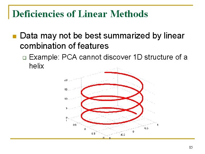
Deficiencies of Linear Methods n Data may not be best summarized by linear combination of features q Example: PCA cannot discover 1 D structure of a helix 85

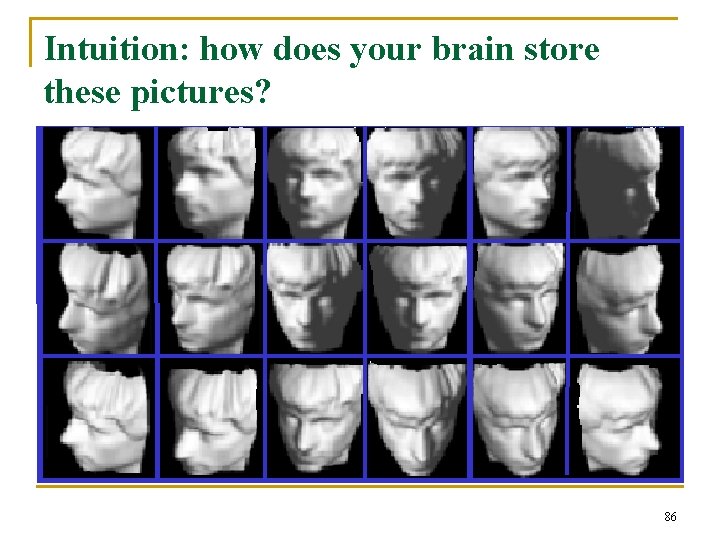
Intuition: how does your brain store these pictures? 86

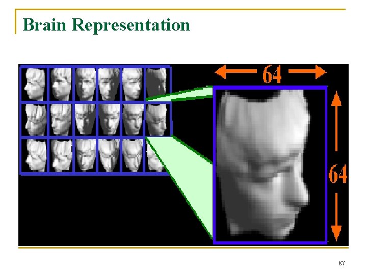
Brain Representation 87

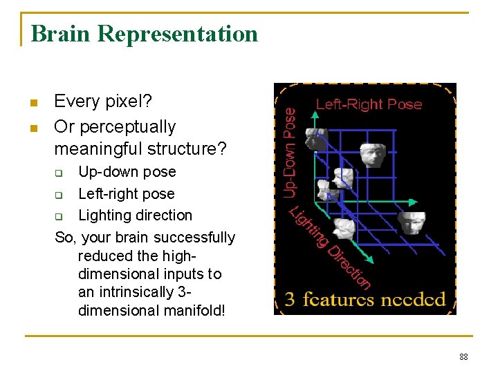
Brain Representation n n Every pixel? Or perceptually meaningful structure? Up-down pose q Left-right pose q Lighting direction So, your brain successfully reduced the highdimensional inputs to an intrinsically 3 dimensional manifold! q 88

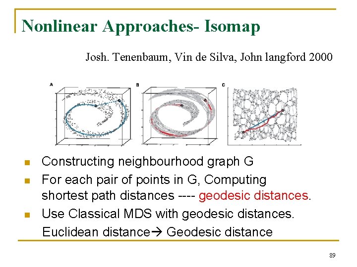
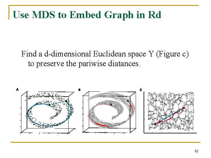
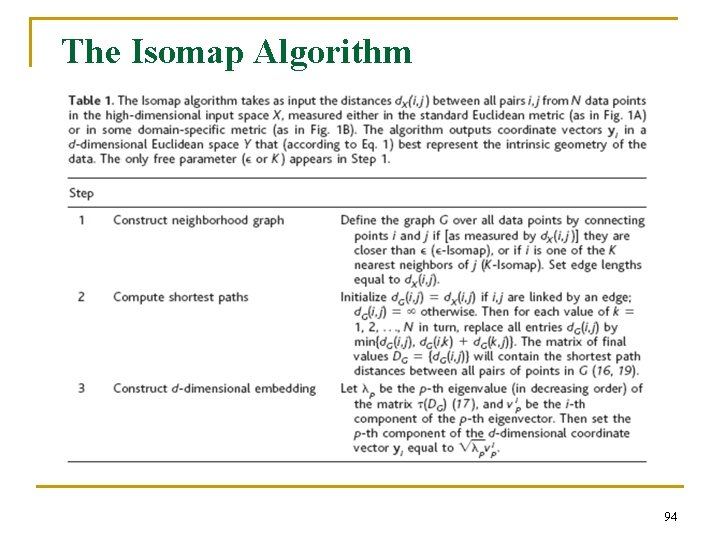
Nonlinear Approaches- Isomap Josh. Tenenbaum, Vin de Silva, John langford 2000 Constructing neighbourhood graph G n For each pair of points in G, Computing shortest path distances ---- geodesic distances. n Use Classical MDS with geodesic distances. Euclidean distance Geodesic distance n 89

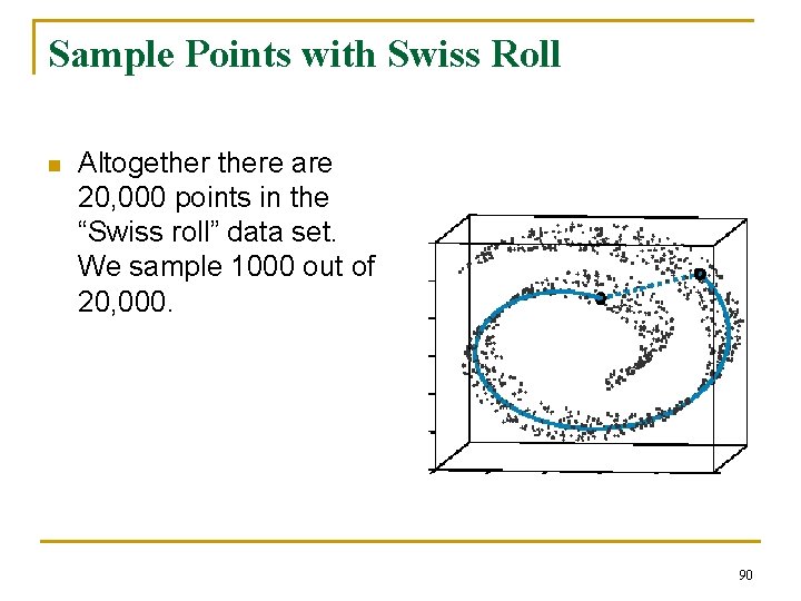
Sample Points with Swiss Roll n Altogethere are 20, 000 points in the “Swiss roll” data set. We sample 1000 out of 20, 000. 90

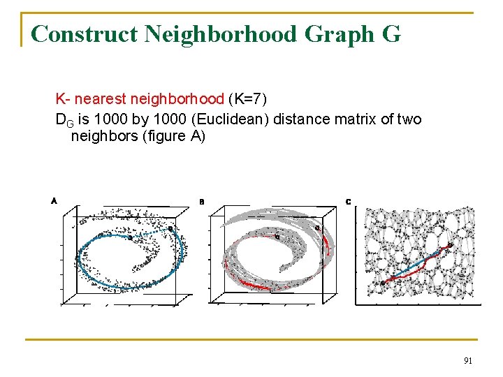
Construct Neighborhood Graph G K- nearest neighborhood (K=7) DG is 1000 by 1000 (Euclidean) distance matrix of two neighbors (figure A) 91

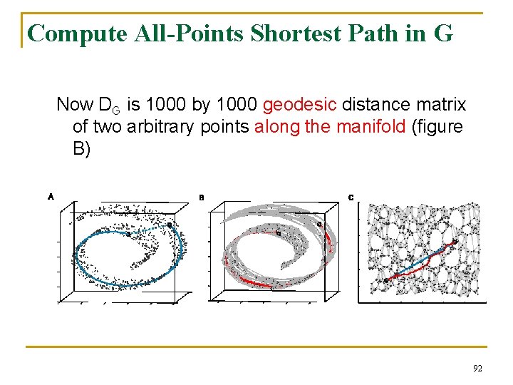
Compute All-Points Shortest Path in G Now DG is 1000 by 1000 geodesic distance matrix of two arbitrary points along the manifold (figure B) 92

Use MDS to Embed Graph in Rd Find a d-dimensional Euclidean space Y (Figure c) to preserve the pariwise diatances. 93

The Isomap Algorithm 94

Isomap: Advantages • Nonlinear • Globally optimal • Still produces globally optimal low-dimensional Euclidean representation even though input space is highly folded, twisted, or curved. • Guarantee asymptotically to recover the true dimensionality. 95

Isomap: Disadvantages • May not be stable, dependent on topology of data • Guaranteed asymptotically to recover geometric structure of nonlinear manifolds – As N increases, pairwise distances provide better approximations to geodesics, but cost more computation – If N is small, geodesic distances will be very inaccurate. 96

Characterictics of a Manifold Rn M z Locally it is a linear patch Key: how to combine all local patches together? R 2 x: coordinate for z x x 1 97

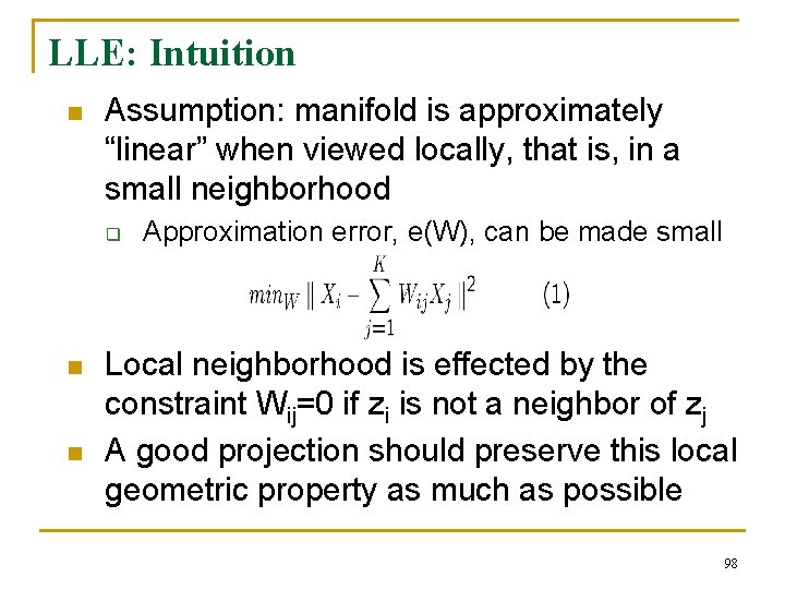
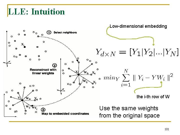
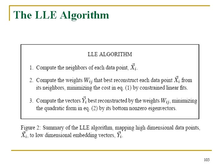
LLE: Intuition n Assumption: manifold is approximately “linear” when viewed locally, that is, in a small neighborhood q n n Approximation error, e(W), can be made small Local neighborhood is effected by the constraint Wij=0 if zi is not a neighbor of zj A good projection should preserve this local geometric property as much as possible 98

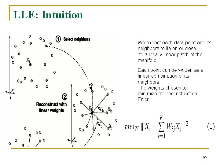
LLE: Intuition We expect each data point and its neighbors to lie on or close to a locally linear patch of the manifold. Each point can be written as a linear combination of its neighbors. The weights chosen to minimize the reconstruction Error. 99

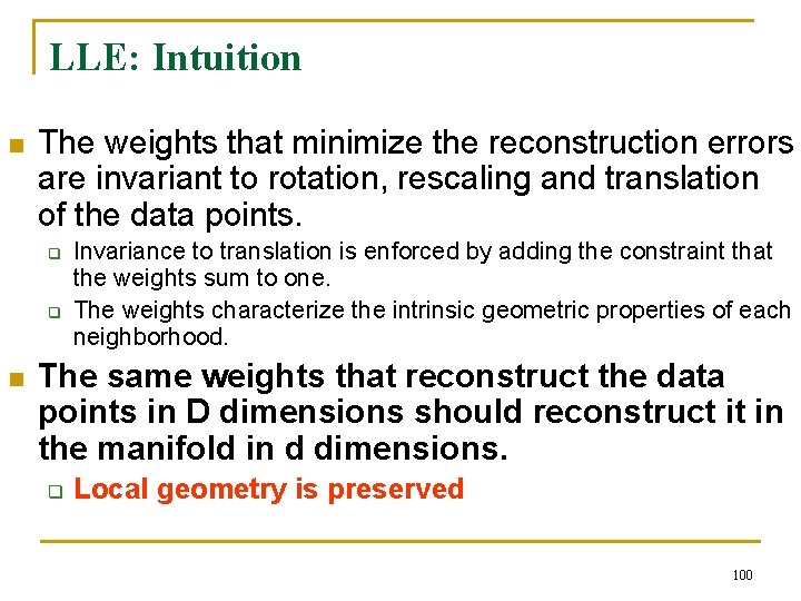
LLE: Intuition n The weights that minimize the reconstruction errors are invariant to rotation, rescaling and translation of the data points. q q n Invariance to translation is enforced by adding the constraint that the weights sum to one. The weights characterize the intrinsic geometric properties of each neighborhood. The same weights that reconstruct the data points in D dimensions should reconstruct it in the manifold in d dimensions. q Local geometry is preserved 100

LLE: Intuition Low-dimensional embedding the i-th row of W Use the same weights from the original space 101

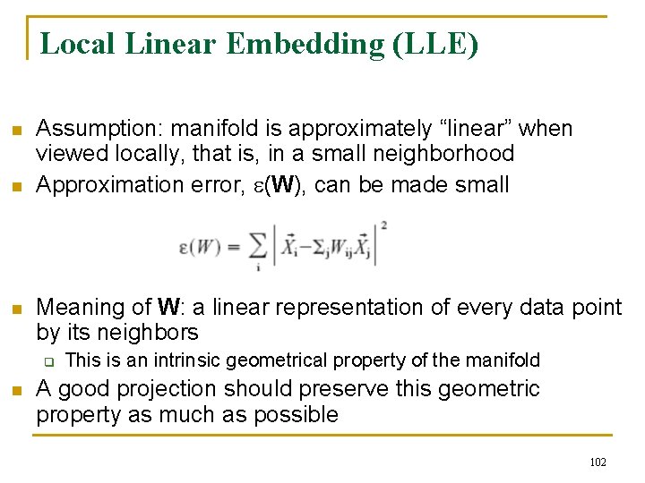
Local Linear Embedding (LLE) n n n Assumption: manifold is approximately “linear” when viewed locally, that is, in a small neighborhood Approximation error, e(W), can be made small Meaning of W: a linear representation of every data point by its neighbors q n This is an intrinsic geometrical property of the manifold A good projection should preserve this geometric property as much as possible 102

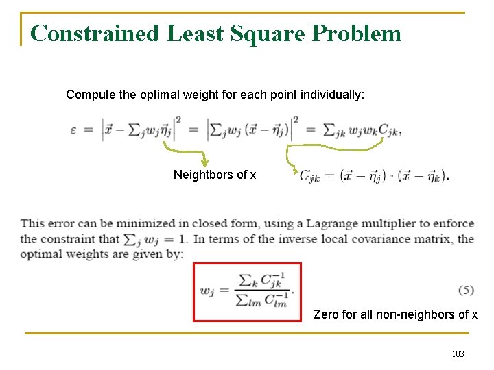
Constrained Least Square Problem Compute the optimal weight for each point individually: Neightbors of x Zero for all non-neighbors of x 103

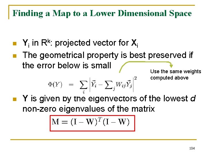
Finding a Map to a Lower Dimensional Space n n Yi in Rk: projected vector for Xi The geometrical property is best preserved if the error below is small Use the same weights computed above n Y is given by the eigenvectors of the lowest d non-zero eigenvalues of the matrix 104

The LLE Algorithm 105

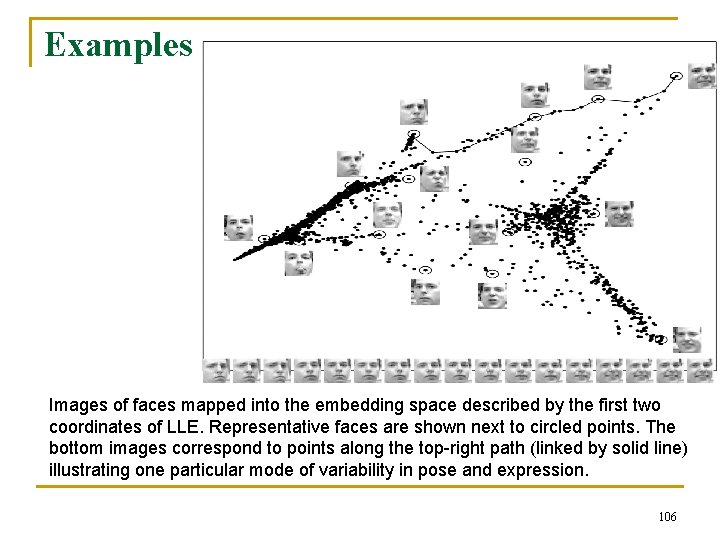
Examples Images of faces mapped into the embedding space described by the first two coordinates of LLE. Representative faces are shown next to circled points. The bottom images correspond to points along the top-right path (linked by solid line) illustrating one particular mode of variability in pose and expression. 106

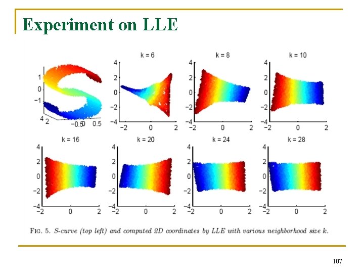
Experiment on LLE 107

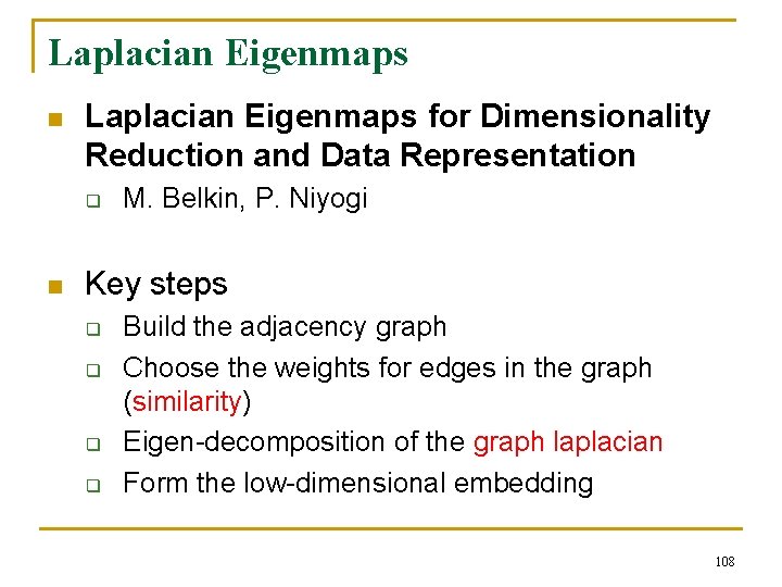
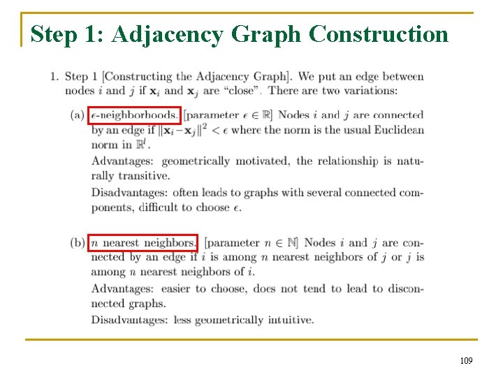
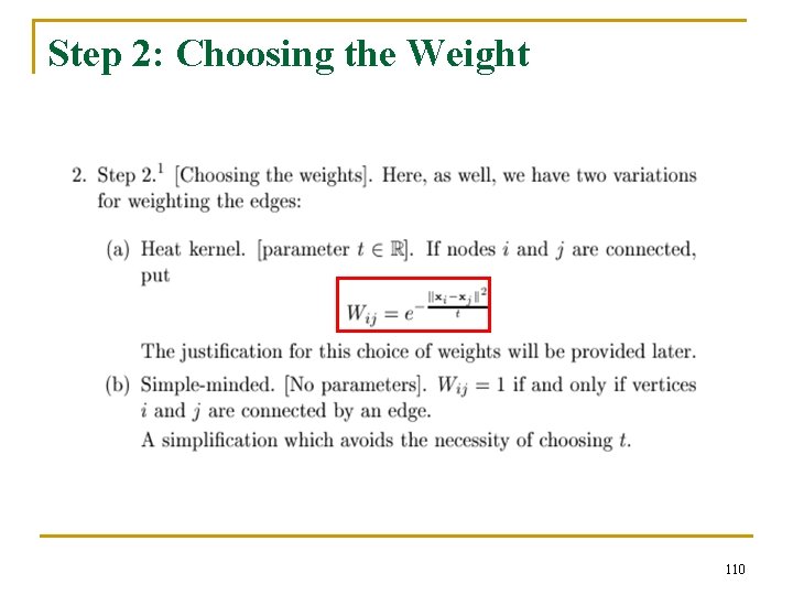
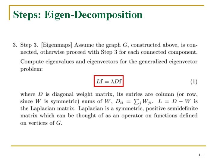
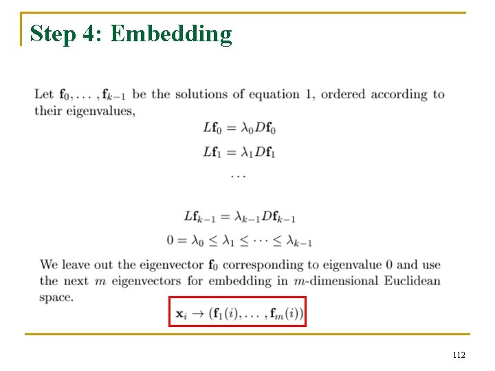
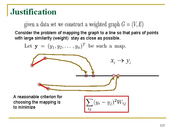
Laplacian Eigenmaps n Laplacian Eigenmaps for Dimensionality Reduction and Data Representation q n M. Belkin, P. Niyogi Key steps q q Build the adjacency graph Choose the weights for edges in the graph (similarity) Eigen-decomposition of the graph laplacian Form the low-dimensional embedding 108

Step 1: Adjacency Graph Construction 109

Step 2: Choosing the Weight 110

Steps: Eigen-Decomposition 111

Step 4: Embedding 112

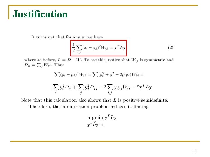
Justification Consider the problem of mapping the graph to a line so that pairs of points with large similarity (weight) stay as close as possible. A reasonable criterion for choosing the mapping is to minimize 113

Justification 114

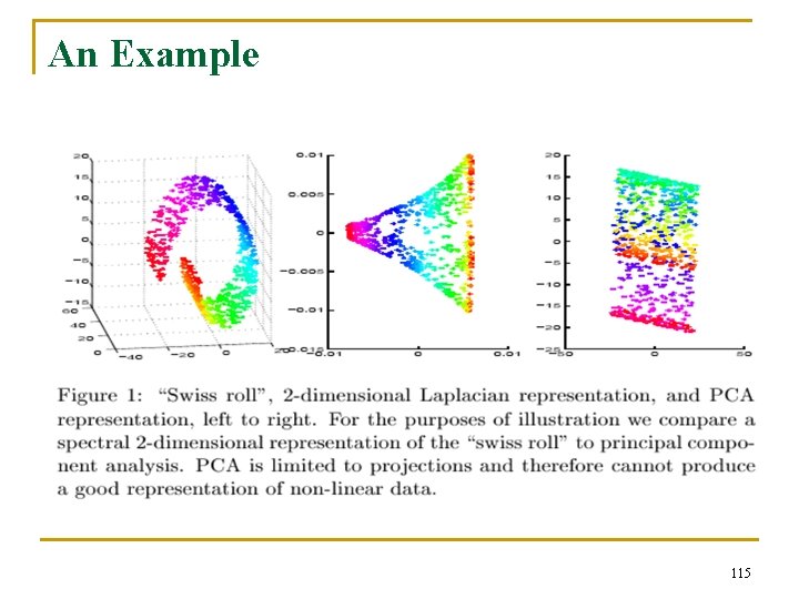
An Example 115

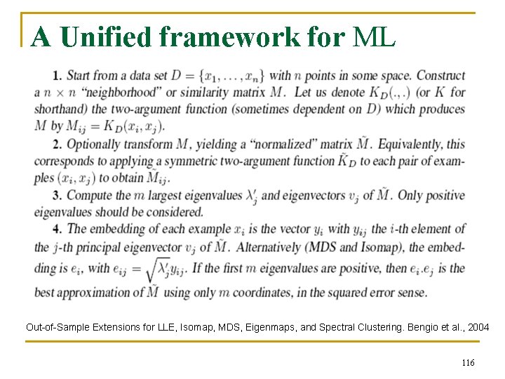
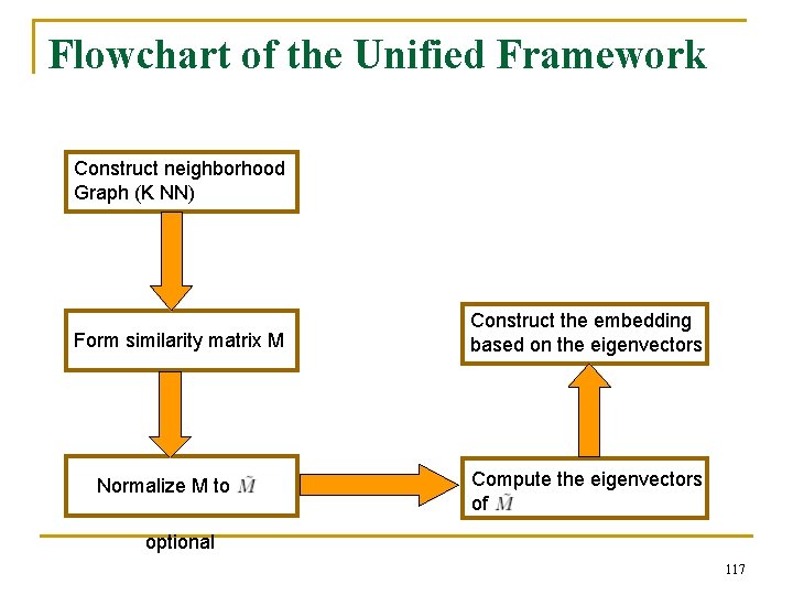
A Unified framework for ML Out-of-Sample Extensions for LLE, Isomap, MDS, Eigenmaps, and Spectral Clustering. Bengio et al. , 2004 116

Flowchart of the Unified Framework Construct neighborhood Graph (K NN) Form similarity matrix M Normalize M to Construct the embedding based on the eigenvectors Compute the eigenvectors of optional 117

Outline n n n Introduction to dimensionality reduction Feature selection (part I) Feature extraction (part II) q q n Basics Representative algorithms Recent advances Applications Recent trends in dimensionality reduction 118

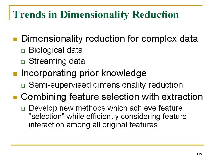
Trends in Dimensionality Reduction n Dimensionality reduction for complex data q q n Incorporating prior knowledge q n Biological data Streaming data Semi-supervised dimensionality reduction Combining feature selection with extraction q Develop new methods which achieve feature “selection” while efficiently considering feature interaction among all original features 119

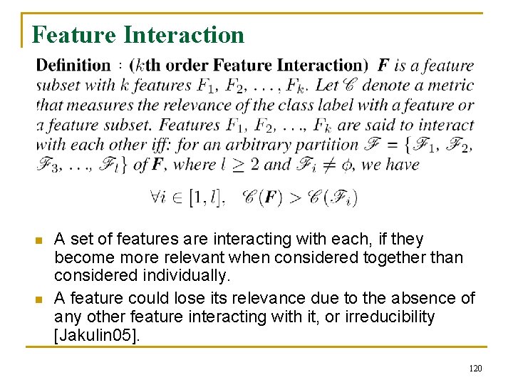
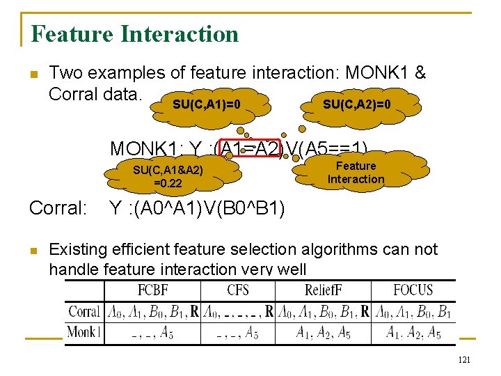
Feature Interaction : n n A set of features are interacting with each, if they become more relevant when considered together than considered individually. A feature could lose its relevance due to the absence of any other feature interacting with it, or irreducibility [Jakulin 05]. 120

Feature Interaction n Two examples of feature interaction: MONK 1 & Corral data. SU(C, A 1)=0 SU(C, A 2)=0 MONK 1: Y : (A 1=A 2)V(A 5==1) SU(C, A 1&A 2) =0. 22 Feature Interaction Corral: Y : (A 0^A 1)V(B 0^B 1) n Existing efficient feature selection algorithms can not handle feature interaction very well 121

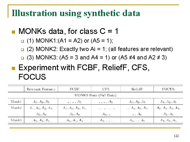
Illustration using synthetic data n MONKs data, for class C = 1 q q q n (1) MONK 1: (A 1 = A 2) or (A 5 = 1); (2) MONK 2: Exactly two Ai = 1; (all features are relevant) (3) MONK 3: (A 5 = 3 and A 4 = 1) or (A 5 ≠ 4 and A 2 ≠ 3) Experiment with FCBF, Relief. F, CFS, FOCUS 122

Existing Solutions for Feature Interaction n n Existing efficient feature selection algorithms usually assume feature independence. Others attempt to explicitly address Feature Interactions by finding them. q n Find out all Feature Interaction is impractical. Some existing efficient algorithm can only (partially) address low order Feature Interaction, 2 or 3 -way Feature Interaction. 123

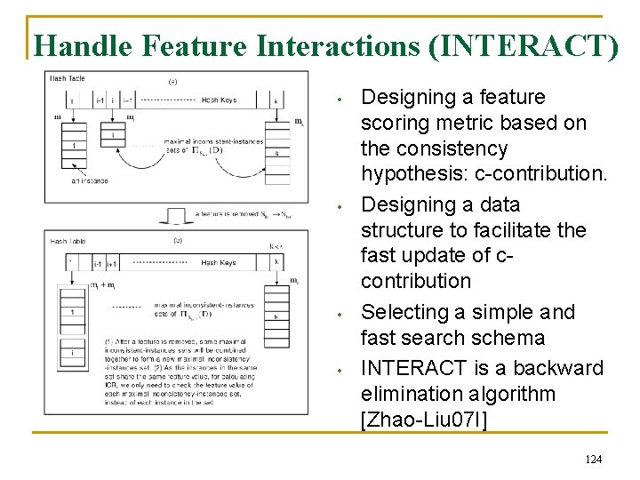
Handle Feature Interactions (INTERACT) • • Designing a feature scoring metric based on the consistency hypothesis: c-contribution. Designing a data structure to facilitate the fast update of ccontribution Selecting a simple and fast search schema INTERACT is a backward elimination algorithm [Zhao-Liu 07 I] 124

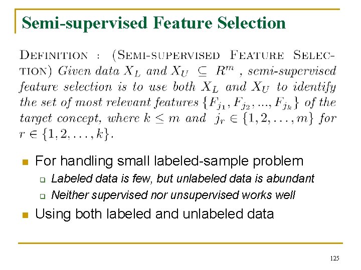
Semi-supervised Feature Selection : n For handling small labeled-sample problem q q n Labeled data is few, but unlabeled data is abundant Neither supervised nor unsupervised works well Using both labeled and unlabeled data 125

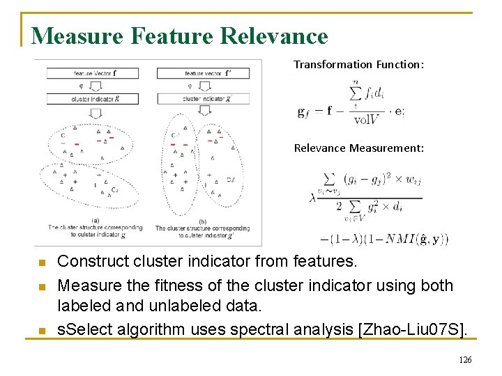
Measure Feature Relevance Transformation Function: Relevance Measurement: n n n Construct cluster indicator from features. Measure the fitness of the cluster indicator using both labeled and unlabeled data. s. Select algorithm uses spectral analysis [Zhao-Liu 07 S]. 126

References 127

References 128

References 129

References 130

References 131

References 132

References 133

References 134

Reference n n n Z. Zhao, H. Liu, Searching for Interacting Features, IJCAI 2007 A. Jakulin, Machine learning based on attribute interactions, Ph. D. thesis, University of Ljubljana 2005. Z. Zhao, H. Liu, Semi-supervised Feature Selection via Spectral Analysis, SDM 2007 135