CS 412 Intro to Data Mining Chapter 3

CS 412 Intro. to Data Mining Chapter 3. Data Preprocessing Qi Li Computer Science, Univ. Illinois at Urbana-Champaign, 2019 1

Chapter 3: Data Preprocessing q Data Preprocessing: An Overview q Data Cleaning q Data Integration q Data Reduction and Transformation q Dimensionality Reduction q Summary 2

Why Preprocess Data? 3 q Raw data not ready to analyze q Issues of data quality q Conclusions drawn may be questionable or unreliable

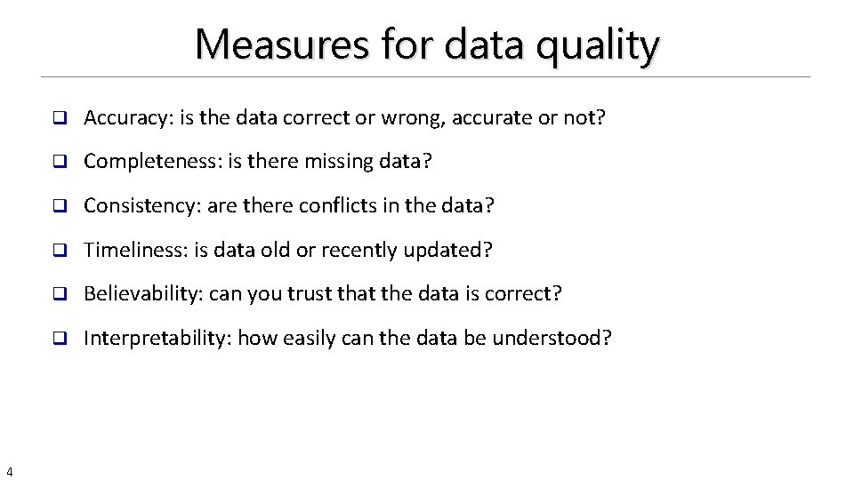
Measures for data quality 4 q Accuracy: is the data correct or wrong, accurate or not? q Completeness: is there missing data? q Consistency: are there conflicts in the data? q Timeliness: is data old or recently updated? q Believability: can you trust that the data is correct? q Interpretability: how easily can the data be understood?

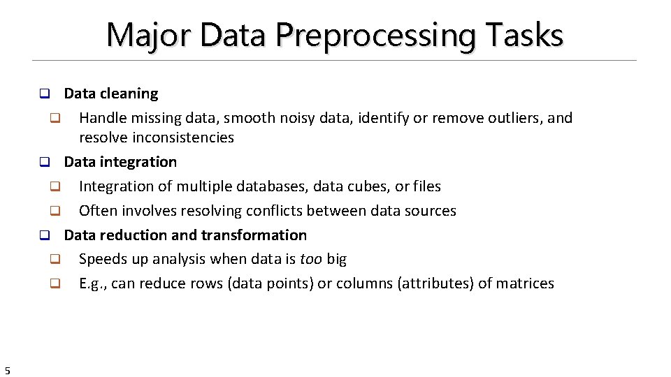
Major Data Preprocessing Tasks Data cleaning q Handle missing data, smooth noisy data, identify or remove outliers, and resolve inconsistencies q Data integration q Integration of multiple databases, data cubes, or files q Often involves resolving conflicts between data sources q Data reduction and transformation q Speeds up analysis when data is too big q E. g. , can reduce rows (data points) or columns (attributes) of matrices q 5

Chapter 3: Data Preprocessing q Data Preprocessing: An Overview q Data Cleaning q Data Integration q Data Reduction and Transformation q Dimensionality Reduction q Summary 6

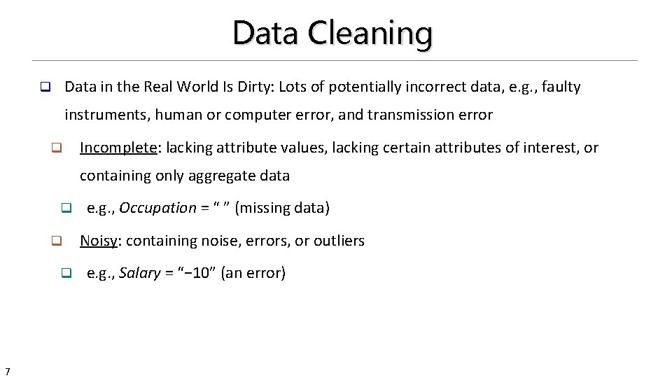
Data Cleaning Data in the Real World Is Dirty: Lots of potentially incorrect data, e. g. , faulty q instruments, human or computer error, and transmission error q Incomplete: lacking attribute values, lacking certain attributes of interest, or containing only aggregate data q q q 7 e. g. , Occupation = “ ” (missing data) Noisy: containing noise, errors, or outliers e. g. , Salary = “− 10” (an error)

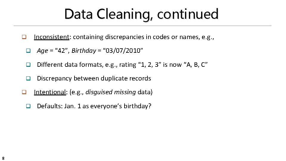
Data Cleaning, continued q q Age = “ 42”, Birthday = “ 03/07/2010” q Different data formats, e. g. , rating “ 1, 2, 3” is now “A, B, C” q Discrepancy between duplicate records q q 8 Inconsistent: containing discrepancies in codes or names, e. g. , Intentional: (e. g. , disguised missing data) Defaults: Jan. 1 as everyone’s birthday?

Incomplete (Missing) Data q q q E. g. , many tuples have no recorded value for several attributes, such as customer income in sales data Missing data may be due to q Equipment malfunction q Inconsistent with other recorded data and thus deleted q Data were not entered due to misunderstanding q Certain data may not be considered important at the time of entry q Did not register history or changes of the data q 9 Data is not always available Missing data may need to be inferred

How to Handle Missing Data? q q q 10 Ignore the tuple Often not desirable, can cause data set to shrink dramatically Fill in the missing value manually Tedious + infeasible? Fill in it automatically with q a global constant : e. g. , “unknown”, a new class? ! q the attribute mean for all samples belonging to the same class: smarter q the most probable value: inference-based such as Bayesian formula or decision tree

Handling Missing Data: Example 11 q Want to predict likely value for missing data q Example: Student missing data for final course grade q This student is male, age 33, 4. 0 GPA q Find similar people in the data and see what their value for final grade is q Fill missing spot with most likely final grade based on the other data

Noisy Data Noise: random error or variance in a measured variable q Incorrect attribute values may be due to various reasons q Faulty data collection instruments, Data entry problems, Data transmission problems, Technology limitation, Inconsistency in naming convention, … q Other data problems q Outliers q Duplicate records q Incomplete data q Inconsistent data q 12

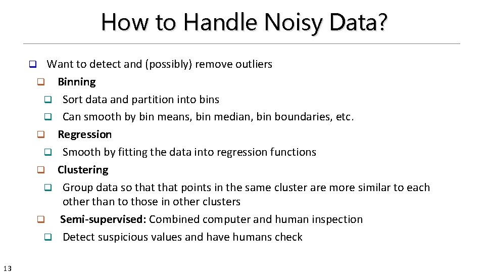
How to Handle Noisy Data? Want to detect and (possibly) remove outliers q Binning q Sort data and partition into bins q Can smooth by bin means, bin median, bin boundaries, etc. q Regression q Smooth by fitting the data into regression functions q Clustering q Group data so that points in the same cluster are more similar to each other than to those in other clusters q Semi-supervised: Combined computer and human inspection q Detect suspicious values and have humans check q 13

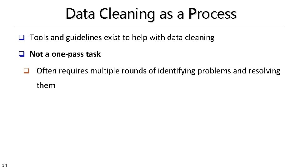
Data Cleaning as a Process q Tools and guidelines exist to help with data cleaning q Not a one-pass task q Often requires multiple rounds of identifying problems and resolving them 14

Chapter 3: Data Preprocessing q Data Preprocessing: An Overview q Data Cleaning q Data Integration q Data Reduction and Transformation q Dimensionality Reduction q Summary 15

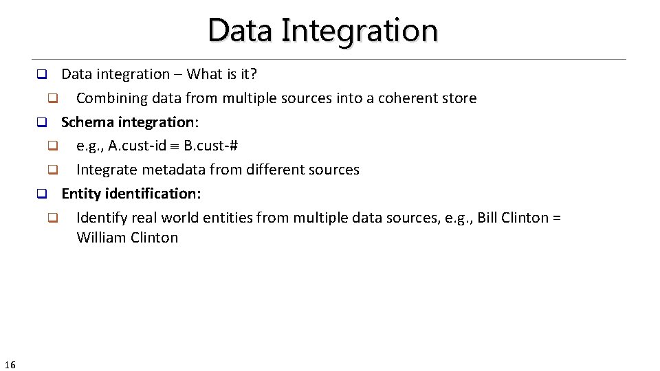
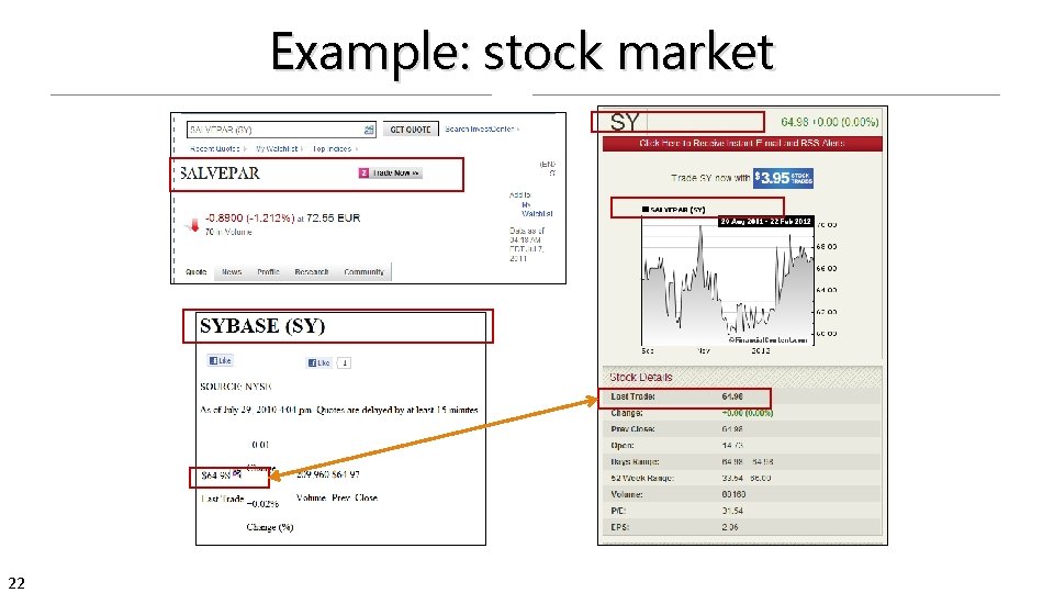
Data Integration Data integration – What is it? q Combining data from multiple sources into a coherent store q Schema integration: q e. g. , A. cust-id B. cust-# q Integrate metadata from different sources q Entity identification: q Identify real world entities from multiple data sources, e. g. , Bill Clinton = William Clinton q 16

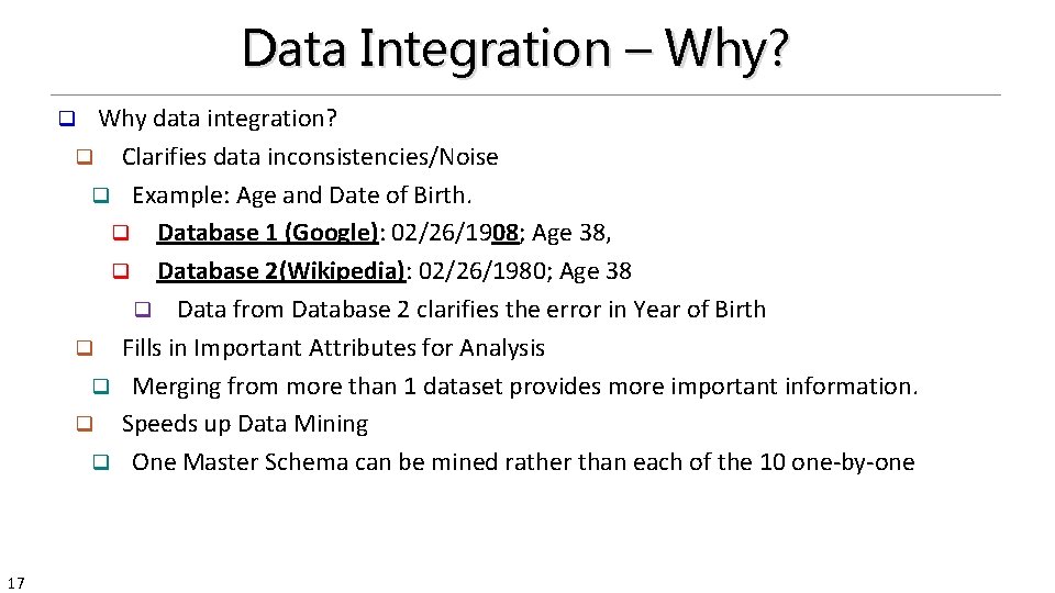
Data Integration – Why? Why data integration? q Clarifies data inconsistencies/Noise q Example: Age and Date of Birth. q Database 1 (Google): 02/26/1908; Age 38, q Database 2(Wikipedia): 02/26/1980; Age 38 q Data from Database 2 clarifies the error in Year of Birth q Fills in Important Attributes for Analysis q Merging from more than 1 dataset provides more important information. q Speeds up Data Mining q One Master Schema can be mined rather than each of the 10 one-by-one q 17

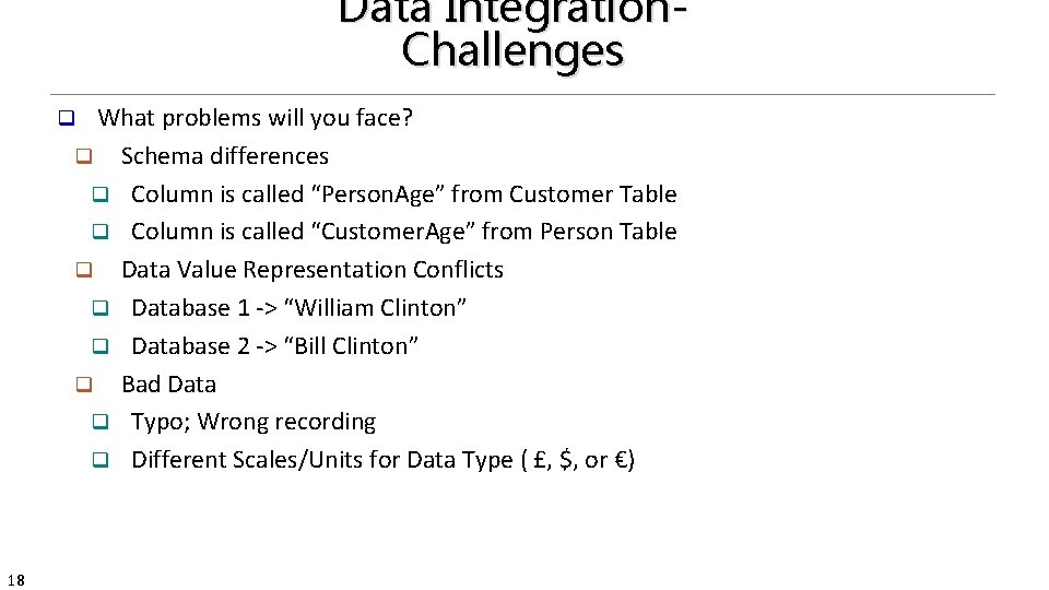
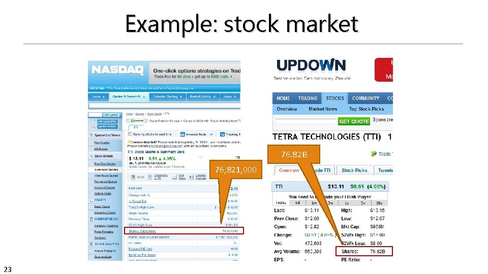
Data Integration. Challenges What problems will you face? q Schema differences q Column is called “Person. Age” from Customer Table q Column is called “Customer. Age” from Person Table q Data Value Representation Conflicts q Database 1 -> “William Clinton” q Database 2 -> “Bill Clinton” q Bad Data q Typo; Wrong recording q Different Scales/Units for Data Type ( £, $, or €) q 18

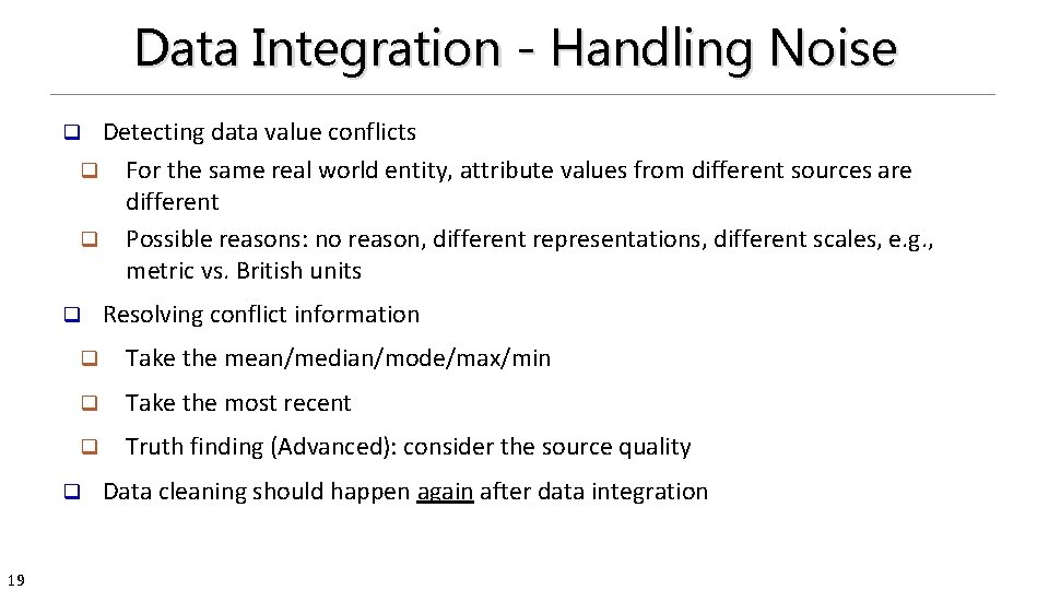
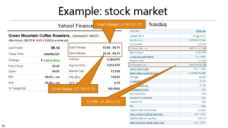
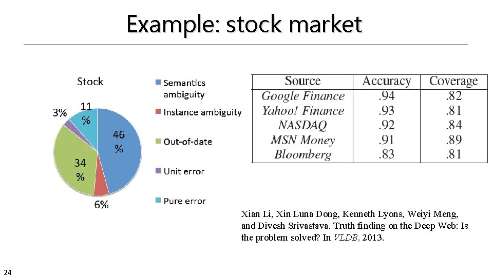
Data Integration - Handling Noise Detecting data value conflicts q For the same real world entity, attribute values from different sources are different q Possible reasons: no reason, different representations, different scales, e. g. , metric vs. British units q q q Take the mean/median/mode/max/min q Take the most recent q Truth finding (Advanced): consider the source quality q 19 Resolving conflict information Data cleaning should happen again after data integration

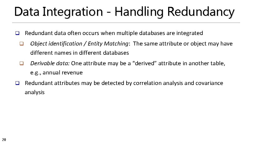
Data Integration - Handling Redundancy q q Object identification / Entity Matching: The same attribute or object may have different names in different databases q Derivable data: One attribute may be a “derived” attribute in another table, e. g. , annual revenue q 20 Redundant data often occurs when multiple databases are integrated Redundant attributes may be detected by correlation analysis and covariance analysis

Example: stock market Yahoo! Finance Day’s Range: 93. 80 -95. 71 52 wk Range: 25. 38 -95. 71 52 Wk: 25. 38 -93. 72 21 Nasdaq

Example: stock market 22

Example: stock market 76. 82 B 76, 821, 000 23

Example: stock market Xian Li, Xin Luna Dong, Kenneth Lyons, Weiyi Meng, and Divesh Srivastava. Truth finding on the Deep Web: Is the problem solved? In VLDB, 2013. 24

Chapter 3: Data Preprocessing q Data Preprocessing: An Overview q Data Cleaning q Data Integration q Data Reduction and Transformation q Dimensionality Reduction q Summary 25

Data Reduction q Data reduction (https: //en. wikipedia. org/wiki/Data_reduction): q q Why data reduction? q q 26 The transformation of data into a simplified or more meaningful form. Data is too big, which causes analysis to be a pain. Example: Large Gigabytes of Data: Forced to chunk/analyze 1 chunk at a time, which is time consuming.

Data Reduction – Row and Column Smart Data Reduction q Attribute Elimination (Column Reduction) q q Throw away useless attributes. q q Throw out “has. ASibling” attribute, and keep “sibling. Has. Disease. A” attribute? Entity Elimination (Row Reduction) q q Example: Find citizens income. Do you need everyone’s income to do this analysis? q 27 Example: Predict if patient will get Disease A Smart Reduction

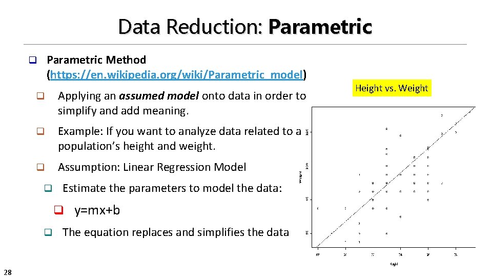
Data Reduction: Parametric Method (https: //en. wikipedia. org/wiki/Parametric_model) q q Applying an assumed model onto data in order to simplify and add meaning. q Example: If you want to analyze data related to a population’s height and weight. q Assumption: Linear Regression Model q Estimate the parameters to model the data: q q 28 y=mx+b The equation replaces and simplifies the data Height vs. Weight

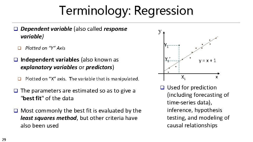
Terminology: Regression q Dependent variable (also called response variable) q q Y 1 Independent variables (also known as explanatory variables or predictors) q 29 Plotted on “Y” Axis y Y 1 ’ X 1 Plotted on “X” axis. The variable that is manipulated. q The parameters are estimated so as to give a "best fit" of the data q Most commonly the best fit is evaluated by the least squares method, but other criteria have also been used y = x + 1 q x Used for prediction (including forecasting of time-series data), inference, hypothesis testing, and modeling of causal relationships

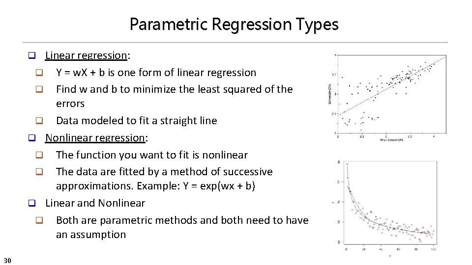
Parametric Regression Types Linear regression: q Y = w. X + b is one form of linear regression q Find w and b to minimize the least squared of the errors q Data modeled to fit a straight line q Nonlinear regression: q The function you want to fit is nonlinear q The data are fitted by a method of successive approximations. Example: Y = exp(wx + b) q Linear and Nonlinear q Both are parametric methods and both need to have an assumption q 30

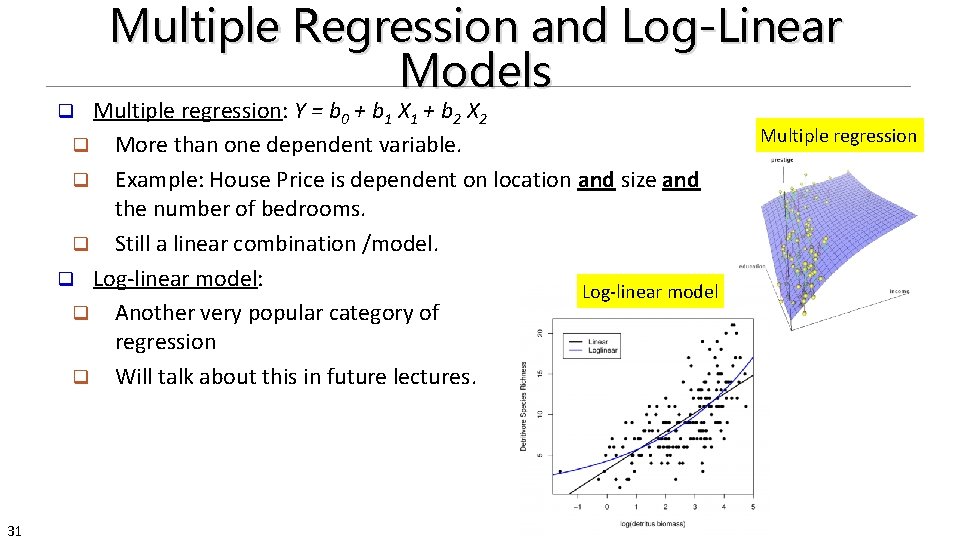
Multiple Regression and Log-Linear Models Multiple regression: Y = b 0 + b 1 X 1 + b 2 X 2 q More than one dependent variable. q Example: House Price is dependent on location and size and the number of bedrooms. q Still a linear combination /model. q Log-linear model: Log-linear model q Another very popular category of regression q Will talk about this in future lectures. q 31 Multiple regression

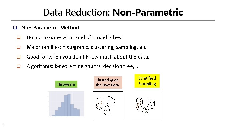
Data Reduction: Non-Parametric q q Do not assume what kind of model is best. q Major families: histograms, clustering, sampling, etc. q Good for when you don’t know much about the data. q Algorithms: k-nearest neighbors, decision tree, … 32 Non-Parametric Method Histogram Clustering on the Raw Data Stratified Sampling

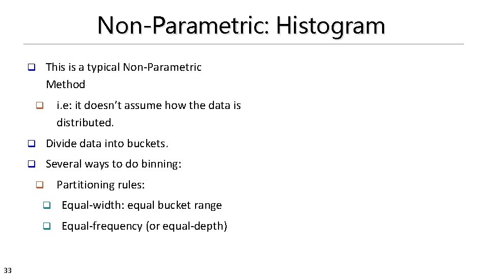
Non-Parametric: Histogram This is a typical Non-Parametric Method q i. e: it doesn’t assume how the data is distributed. q q Divide data into buckets. q Several ways to do binning: q 33 Partitioning rules: q Equal-width: equal bucket range q Equal-frequency (or equal-depth)

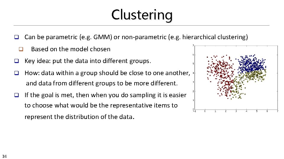
Clustering q q Can be parametric (e. g. GMM) or non-parametric (e. g. hierarchical clustering) Based on the model chosen q Key idea: put the data into different groups. q How: data within a group should be close to one another, and data from different groups to be more different. q If the goal is met, then when you do sampling it is easier to choose what would be the representative items to represent the distribution of the data. 34

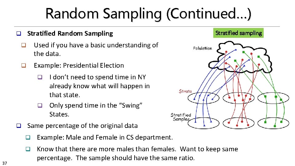
Data Reduction: Sampling q Sampling: obtaining a small sample s to represent the whole data set N q Key principles: q Choose a representative subset and of the data q Choose an appropriate size of the sample q 35 Example: Presidential election q Predicting which candidate will win the final election q Can not pick 1000 s, you need more q Can not only sample people from NY. You need multiple regions

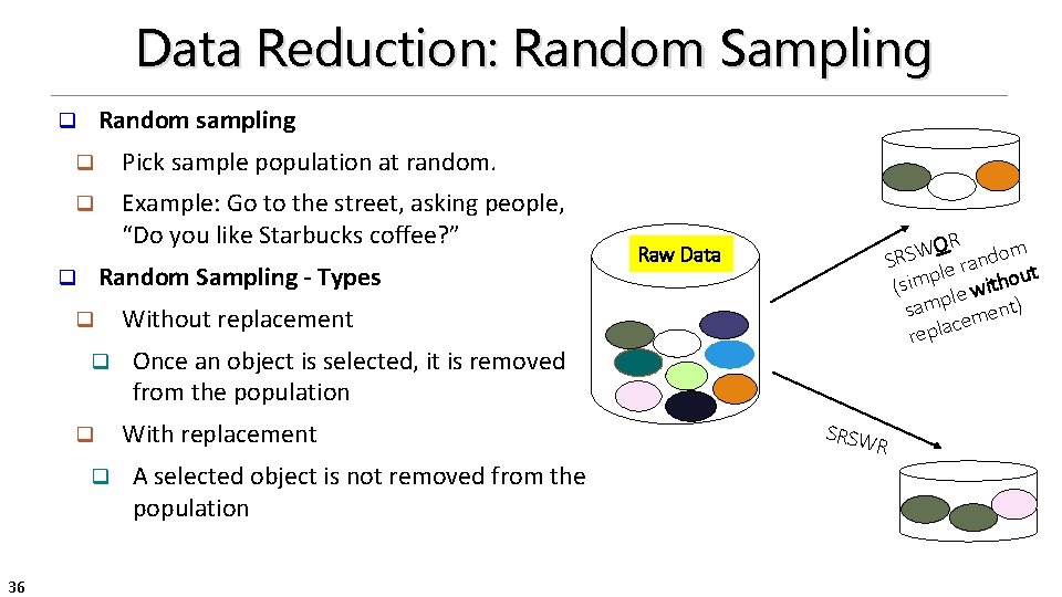
Data Reduction: Random Sampling Random sampling q q Pick sample population at random. q Example: Go to the street, asking people, “Do you like Starbucks coffee? ” Random Sampling - Types q q q 36 OR W S dom R n S a r le p out m i h t s i ( le w t) p m sa en m e c repla Raw Data Without replacement Once an object is selected, it is removed from the population With replacement A selected object is not removed from the population SRSW R

Random Sampling (Continued…) Stratified Random Sampling q q Used if you have a basic understanding of the data. q Example: Presidential Election Stratified sampling I don’t need to spend time in NY already know what will happen in that state. q Only spend time in the “Swing” States. q q 37 Same percentage of the original data q Example: Male and Female in CS department. q Know that there are more males than females. Want to keep same percentage. The sample should have the same ratio.

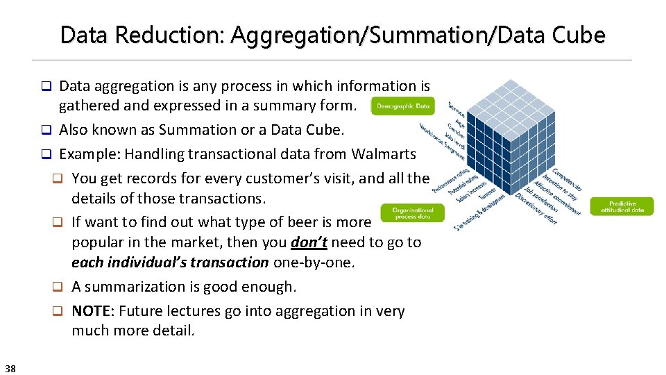
Data Reduction: Aggregation/Summation/Data Cube Data aggregation is any process in which information is gathered and expressed in a summary form. q Also known as Summation or a Data Cube. q Example: Handling transactional data from Walmarts q You get records for every customer’s visit, and all the details of those transactions. q If want to find out what type of beer is more popular in the market, then you don’t need to go to each individual’s transaction one-by-one. q A summarization is good enough. q NOTE: Future lectures go into aggregation in very much more detail. q 38

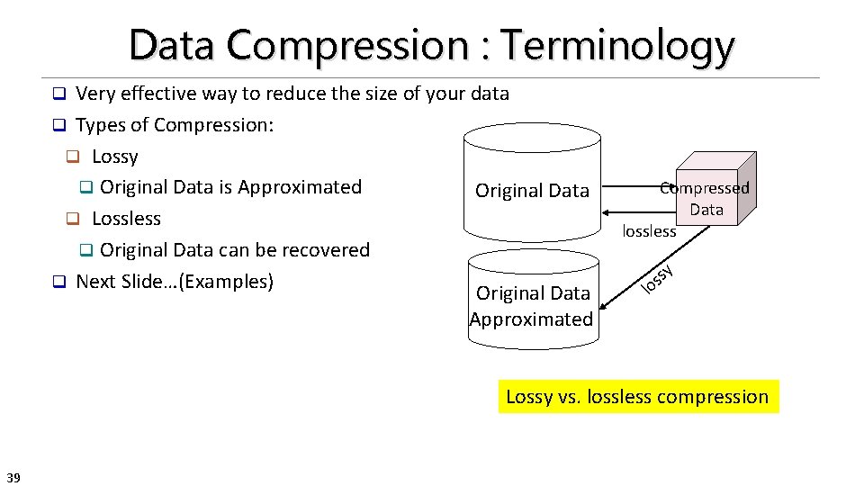
Data Compression : Terminology Very effective way to reduce the size of your data q Types of Compression: q Lossy q Original Data is Approximated Original Data q Lossless q Original Data can be recovered q Next Slide…(Examples) Original Data Approximated q Compressed Data lossless y l s os Lossy vs. lossless compression 39

Data Compression : Lossless vs Lossy q Example: Phone Photo Sample Image q A small photo, less space, gives basic information. q If you think its important, you click download and you get all the data from the web for this image. q The small photo is lossy compression of the bigger image. q Lossless q Example: Zip file. q On unzip, you get the original data. No Data is lost, its just in a different format. q Example: 10 k x 10 k matrix of 1 s and 0 s q Of only 100 are “ 1”, then only store the location of 1 s. q Can easily reconstruct the matrix. No information is lost. q 40

Data Transformation q What is it? q A function that maps the entire set of values of a given attribute to a new set of replacement values q Each old value can be identified with one of the new values q When do I normalize? q If your data already has the same meaning, there is no need to normalize. q q Example: Two data sets: High Temperature, Low Temperature If they have different meanings, then you should normalize to compare them. q Example: Age vs Income. q These are hard to compare because of the range of values in Age is 0 -99 , and income maybe is 12 k – 100 k, etc. 41

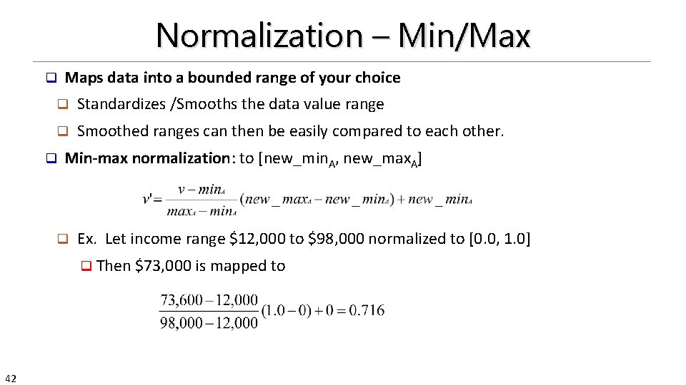
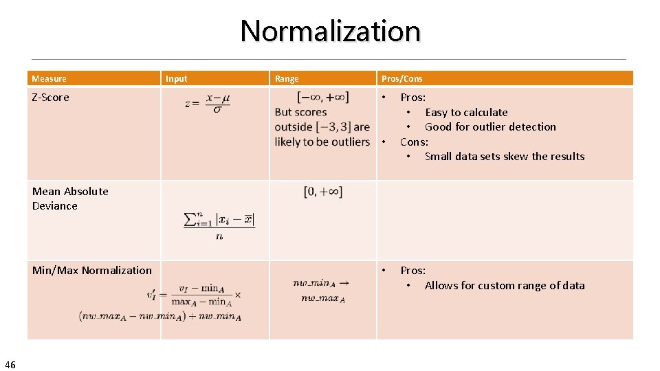
Normalization – Min/Max q Maps data into a bounded range of your choice q Standardizes /Smooths the data value range q Smoothed ranges can then be easily compared to each other. q Min-max normalization: to [new_min. A, new_max. A] q Ex. Let income range $12, 000 to $98, 000 normalized to [0. 0, 1. 0] q Then $73, 000 is mapped to 42

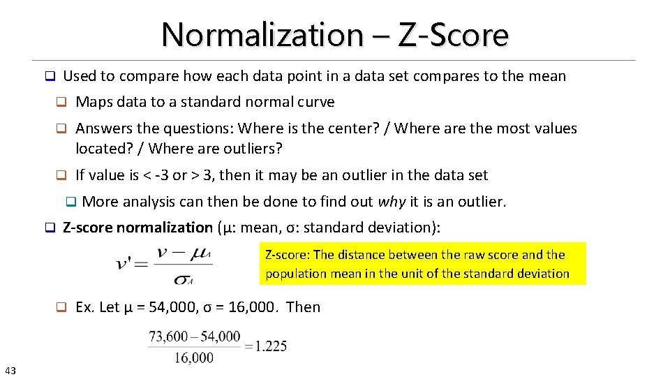
Normalization – Z-Score q Used to compare how each data point in a data set compares to the mean q Maps data to a standard normal curve q Answers the questions: Where is the center? / Where are the most values located? / Where are outliers? q If value is < -3 or > 3, then it may be an outlier in the data set q q More analysis can then be done to find out why it is an outlier. Z-score normalization (μ: mean, σ: standard deviation): Z-score: The distance between the raw score and the population mean in the unit of the standard deviation q 43 Ex. Let μ = 54, 000, σ = 16, 000. Then

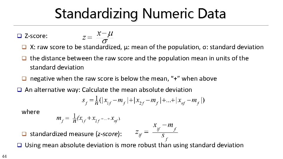
Standardizing Numeric Data q Z-score: q X: raw score to be standardized, μ: mean of the population, σ: standard deviation q the distance between the raw score and the population mean in units of the standard deviation q negative when the raw score is below the mean, “+” when above q An alternative way: Calculate the mean absolute deviation where q q 44 standardized measure (z-score): Using mean absolute deviation is more robust than using standard deviation

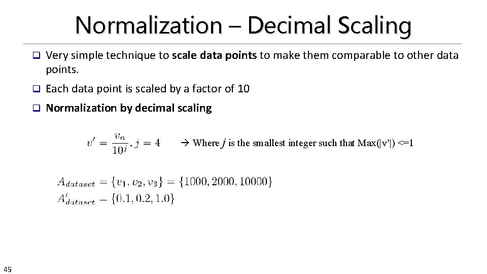
Normalization – Decimal Scaling q Very simple technique to scale data points to make them comparable to other data points. q Each data point is scaled by a factor of 10 q Normalization by decimal scaling Where j is the smallest integer such that Max(|ν’|) <=1 45

Normalization Measure Z-Score Input Range Pros/Cons • • Pros: • Easy to calculate • Good for outlier detection Cons: • Small data sets skew the results Mean Absolute Deviance Min/Max Normalization 46 • Pros: • Allows for custom range of data

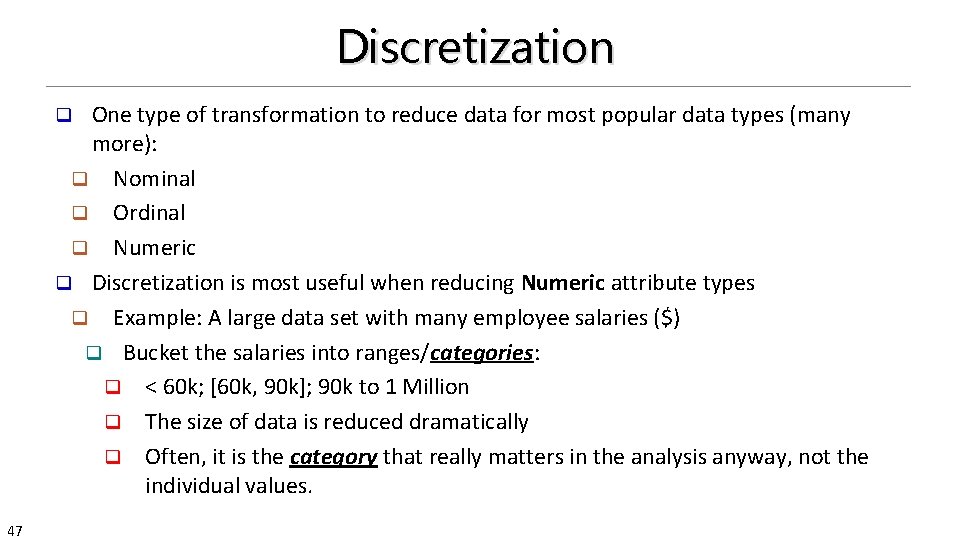
Discretization One type of transformation to reduce data for most popular data types (many more): q Nominal q Ordinal q Numeric q Discretization is most useful when reducing Numeric attribute types q Example: A large data set with many employee salaries ($) q Bucket the salaries into ranges/categories: q < 60 k; [60 k, 90 k]; 90 k to 1 Million q The size of data is reduced dramatically q Often, it is the category that really matters in the analysis anyway, not the individual values. q 47

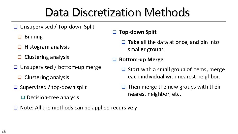
Data Discretization Methods q Unsupervised / Top-down Split q Binning q Histogram analysis q Clustering analysis q Unsupervised / bottom-up merge q q 48 Top-down Split q q Supervised / top-down split Decision-tree analysis Take all the data at once, and bin into smaller groups Bottom-up Merge q Start with a small group of items, merge each individual with nearest neighbor. q Then merge the new groups with their nearest neighbor, etc. Clustering analysis q q q Note: All the methods can be applied recursively

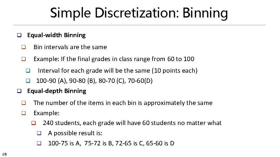
Simple Discretization: Binning Equal-width Binning q q Bin intervals are the same q Example: If the final grades in class range from 60 to 100 Interval for each grade will be the same (10 points each) q 100 -90 (A), 90 -80 (B), 80 -70 (C), 70 -60(D) q Equal-depth Binning q The number of the items in each bin is approximately the same q Example: q 240 students, each grade will have 60 students no matter what q A possible result is: q 100 -75 is A, 75 -72 is B, 72 -65 is C, 65 -60 is D q 49

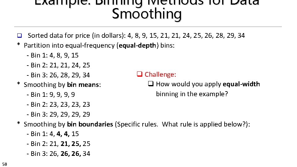
Example: Binning Methods for Data Smoothing Sorted data for price (in dollars): 4, 8, 9, 15, 21, 24, 25, 26, 28, 29, 34 * Partition into equal-frequency (equal-depth) bins: - Bin 1: 4, 8, 9, 15 - Bin 2: 21, 24, 25 q Challenge: - Bin 3: 26, 28, 29, 34 q How would you apply equal-width * Smoothing by bin means: binning in the example? - Bin 1: 9, 9, 9, 9 - Bin 2: 23, 23, 23 - Bin 3: 29, 29, 29 * Smoothing by bin boundaries (Specific rules. What rule is applied below? ): - Bin 1: 4, 4, 4, 15 - Bin 2: 21, 25, 25 - Bin 3: 26, 26, 34 q 50

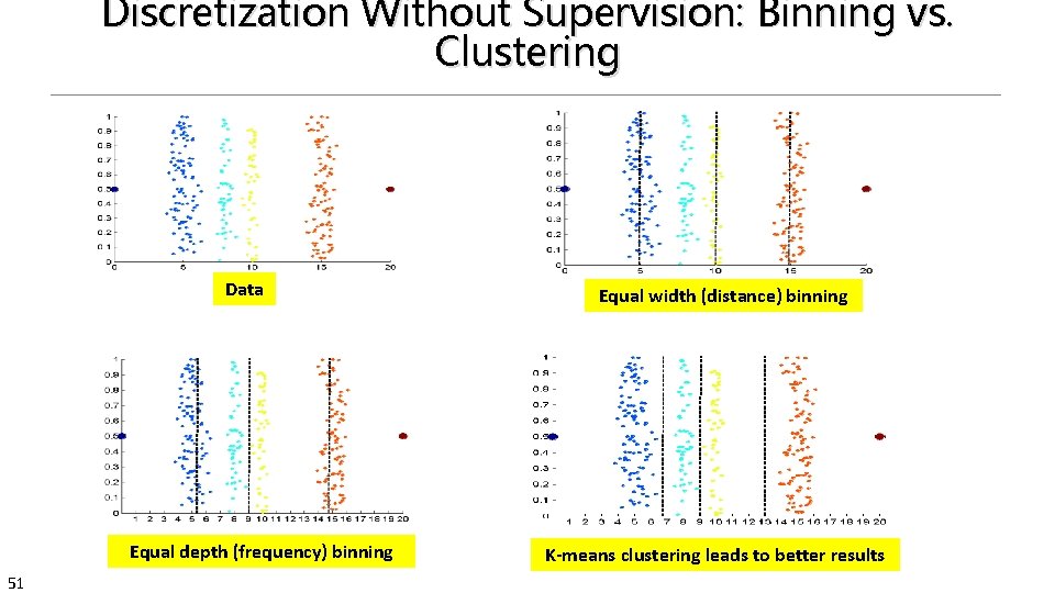
Discretization Without Supervision: Binning vs. Clustering Data Equal depth (frequency) binning 51 Equal width (distance) binning K-means clustering leads to better results

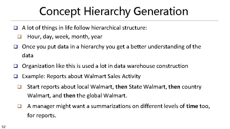
Concept Hierarchy Generation A lot of things in life follow hierarchical structure: q Hour, day, week, month, year q q Once you put data in a hierarchy you get a better understanding of the data q Organization like this is used a lot in data warehouse construction q Example: Reports about Walmart Sales Activity q Start reports about local Walmart, then State Walmart, then country Walmart, and then the global Walmart. q A manager might want a summarizations on different levels of time too, for reports. 52

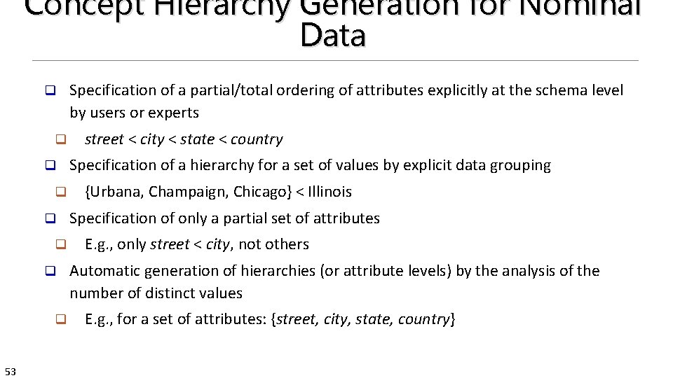
Concept Hierarchy Generation for Nominal Data q q q q 53 Specification of a partial/total ordering of attributes explicitly at the schema level by users or experts street < city < state < country Specification of a hierarchy for a set of values by explicit data grouping {Urbana, Champaign, Chicago} < Illinois Specification of only a partial set of attributes E. g. , only street < city, not others Automatic generation of hierarchies (or attribute levels) by the analysis of the number of distinct values E. g. , for a set of attributes: {street, city, state, country}

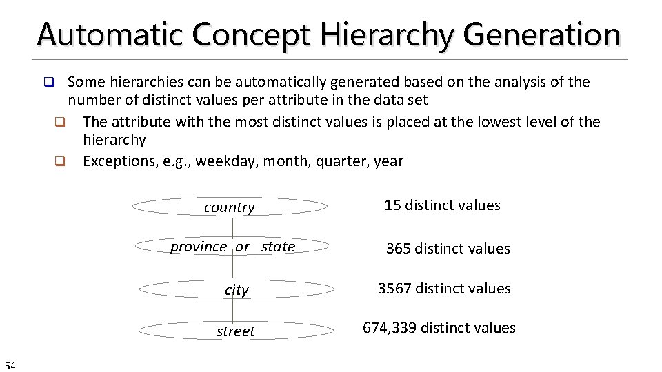
Automatic Concept Hierarchy Generation Some hierarchies can be automatically generated based on the analysis of the number of distinct values per attribute in the data set q The attribute with the most distinct values is placed at the lowest level of the hierarchy q Exceptions, e. g. , weekday, month, quarter, year q country province_or_ state 365 distinct values city 3567 distinct values street 54 15 distinct values 674, 339 distinct values

Chapter 3: Data Preprocessing q Data Preprocessing: An Overview q Data Cleaning q Data Integration q Data Reduction and Transformation q Dimensionality Reduction q Summary 55

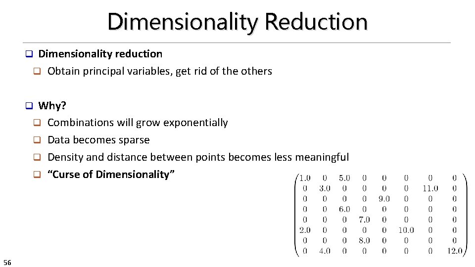
Dimensionality Reduction Dimensionality reduction q Obtain principal variables, get rid of the others q Why? q Combinations will grow exponentially q Data becomes sparse q Density and distance between points becomes less meaningful q “Curse of Dimensionality” q 56

Dimensionality Reduction q Advantages of dimensionality reduction q Avoid the curse of dimensionality q Help eliminate irrelevant features and reduce noise q Reduce time and space required in data mining q Allow easier visualization 57

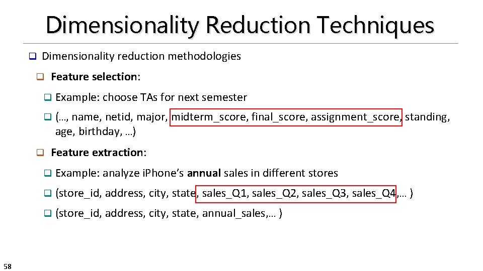
Dimensionality Reduction Techniques q Dimensionality reduction methodologies q q Example: choose TAs for next semester q (…, name, netid, major, midterm_score, final_score, assignment_score, standing, age, birthday, …) q 58 Feature selection: Feature extraction: q Example: analyze i. Phone’s annual sales in different stores q (store_id, address, city, state, sales_Q 1, sales_Q 2, sales_Q 3, sales_Q 4, … ) q (store_id, address, city, state, annual_sales, … )

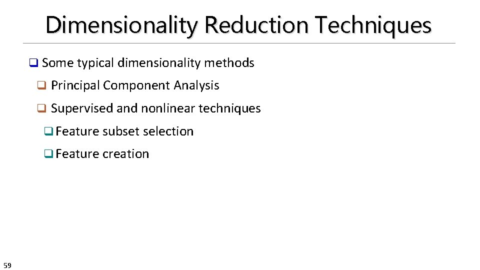
Dimensionality Reduction Techniques q Some typical dimensionality methods q Principal Component Analysis q Supervised and nonlinear techniques q Feature subset selection q Feature creation 59

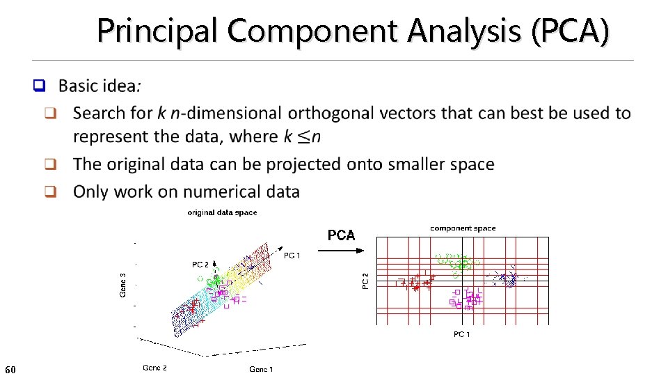
Principal Component Analysis (PCA) q 60

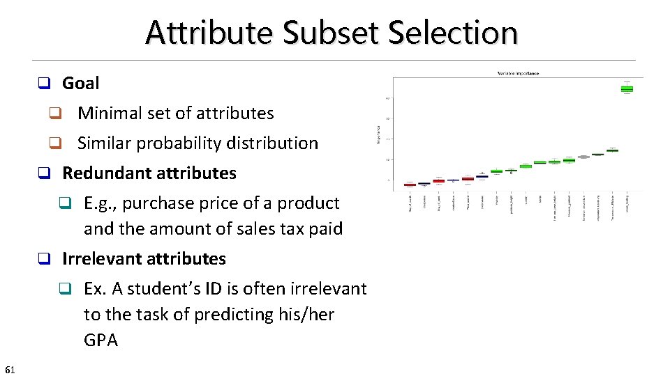
Attribute Subset Selection Goal q q Minimal set of attributes q Similar probability distribution q Redundant attributes q q Irrelevant attributes q 61 E. g. , purchase price of a product and the amount of sales tax paid Ex. A student’s ID is often irrelevant to the task of predicting his/her GPA

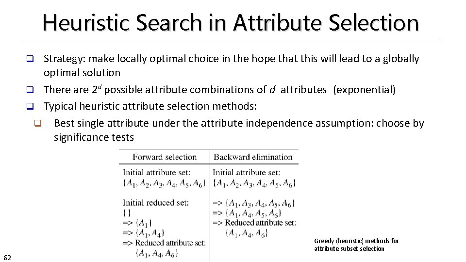
Heuristic Search in Attribute Selection Strategy: make locally optimal choice in the hope that this will lead to a globally optimal solution q There are 2 d possible attribute combinations of d attributes (exponential) q Typical heuristic attribute selection methods: q Best single attribute under the attribute independence assumption: choose by significance tests q 62 Greedy (heuristic) methods for attribute subset selection

Attribute Creation (Feature Generation) Create new attributes (features) that can capture the important information in a data set more effectively than the original ones q Three general methodologies q Attribute extraction q Domain-specific q Mapping data to new space (see: data reduction) q E. g. , Fourier transformation, wavelet transformation, manifold approaches (not covered) q Attribute construction q Combining features (see: discriminative frequent patterns in Chapter on “Advanced Classification”) q Data discretization q 63

Summary q Data quality: accuracy, completeness, consistency, timeliness, believability, interpretability q Data cleaning: e. g. missing/noisy values, outliers q Data integration from multiple sources: q q Data reduction, data transformation and data discretization q Numerosity reduction; Data compression q Normalization; Concept hierarchy generation q 64 Entity identification problem; Remove redundancies; Detect inconsistencies Dimensionality reduction q Feature selection and feature extraction q PCA; attribute subset selection (heuristic search); attribute creation

References q q q q q 65 D. P. Ballou and G. K. Tayi. Enhancing data quality in data warehouse environments. Comm. of ACM, 42: 73 -78, 1999 T. Dasu and T. Johnson. Exploratory Data Mining and Data Cleaning. John Wiley, 2003 T. Dasu, T. Johnson, S. Muthukrishnan, V. Shkapenyuk. Mining Database Structure; Or, How to Build a Data Quality Browser. SIGMOD’ 02 H. V. Jagadish et al. , Special Issue on Data Reduction Techniques. Bulletin of the Technical Committee on Data Engineering, 20(4), Dec. 1997 D. Pyle. Data Preparation for Data Mining. Morgan Kaufmann, 1999 E. Rahm and H. H. Do. Data Cleaning: Problems and Current Approaches. IEEE Bulletin of the Technical Committee on Data Engineering. Vol. 23, No. 4 V. Raman and J. Hellerstein. Potters Wheel: An Interactive Framework for Data Cleaning and Transformation, VLDB’ 2001 T. Redman. Data Quality: Management and Technology. Bantam Books, 1992 R. Wang, V. Storey, and C. Firth. A framework for analysis of data quality research. IEEE Trans. Knowledge and Data Engineering, 7: 623 -640, 1995