Data Mining Concepts and Techniques 3 rd ed

Data Mining: Concepts and Techniques (3 rd ed. ) — Chapter 3 — Jiawei Han, Micheline Kamber, and Jian Pei University of Illinois at Urbana-Champaign & Simon Fraser University © 2010 Han, Kamber & Pei. All rights reserved. 9/9/2020 1

Chapter 3: Data Preprocessing n Data Preprocessing: An Overview n Data Quality n Major Tasks in Data Preprocessing n Data Cleaning n Data Integration n Data Reduction n Data Transformation and Data Discretization n Summary 2

Correlation Analysis (Nominal Data) n n Χ 2 (chi-square) test The larger the Χ 2 value, the more likely the variables are related The cells that contribute the most to the Χ 2 value are those whose actual count is very different from the expected count Correlation does not imply causality n # of hospitals and # of car-theft in a city are correlated n Both are causally linked to the third variable: population 3

Chi-Square Calculation n Suppose A has c distinct values, namely a 1, a 2, …, ac. B has r distinct values, namely b 1, b 2, …, br. (Ai, Bj) denote the event that (A=ai, B=bj) oij is the observed frequency eij is the expected frequency

Chi-Square Calculation n The Χ 2 statistic tests the hypothesis that A and B are independent The test is based on a significance level, with (r 1)(c-1) degrees of freedom If the hypothesis can be rejected, then we say that A and B are statistically related or associated

Chi-Square Calculation: An Example n Suppose that a group of 1, 500 people was surveyed. The gender of each person was noted. Each person was polled as to whether their preferred type of reading material was fiction or nonfiction. Thus, we have two attributes, gender and preferred reading. The observed frequency (or count) of each possible joint event is summarized in the contingency table shown in the table (next slide), where the numbers in parentheses are the expected frequencies.

Chi-Square Calculation: An Example n n male female Sum (row) fiction 250(90) 200(360) 450 non fiction 50(210) 1000(840) 1050 Sum(col. ) 300 1200 1500 Χ 2 (chi-square) calculation (numbers in parenthesis are expected counts calculated based on the data distribution in the two categories) It shows that preferred_reading and gender are correlated in the group

Chi-Square Calculation: An Example n For this 2 2 table, the degrees of freedom are (21)(2 -1) = 1. For 1 degree of freedom, the Χ 2 value needed to reject the hypothesis at the 0. 001 significance level is 10. 828 (taken from the table of upper percentage points of the Χ 2 distribution, typically available from any textbook on statistics). Since our computed value is above this, we can reject the hypothesis that gender and preferred reading are independent and conclude that the two attributes are (strongly) correlated for the given group of people.

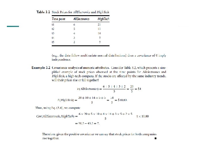
Covariance (Numeric Data) n Covariance is similar to correlation Correlation coefficient: where n is the number of tuples, and are the respective mean or expected values of A and B, σA and σB are the respective standard deviation of A and B. n n n Positive covariance: If Cov. A, B > 0, then A and B both tend to be larger than their expected values. Negative covariance: If Cov. A, B < 0 then if A is larger than its expected value, B is likely to be smaller than its expected value. Independence: Cov. A, B = 0 but the converse is not true: n Some pairs of random variables may have a covariance of 0 but are not independent. Only under some additional assumptions (e. g. , the data follow multivariate normal distributions) does a covariance of 0 imply independence 9

Co-Variance: An Example n It can be simplified in computation as n Suppose two stocks A and B have the following values in one week: (2, 5), (3, 8), (5, 10), (4, 11), (6, 14). n Question: If the stocks are affected by the same industry trends, will their prices rise or fall together? n n E(A) = (2 + 3 + 5 + 4 + 6)/ 5 = 20/5 = 4 n E(B) = (5 + 8 + 10 + 11 + 14) /5 = 48/5 = 9. 6 n Cov(A, B) = (2× 5+3× 8+5× 10+4× 11+6× 14)/5 − 4 × 9. 6 = 4 Thus, A and B rise together since Cov(A, B) > 0.

Chapter 3: Data Preprocessing n Data Preprocessing: An Overview n Data Quality n Major Tasks in Data Preprocessing n Data Cleaning n Data Integration n Data Reduction n Data Transformation and Data Discretization n Summary 12

Data Reduction Strategies n n n Data reduction: Obtain a reduced representation of the data set that is much smaller in volume but yet produces the same (or almost the same) analytical results Why data reduction? — A database/data warehouse may store terabytes of data. Complex data analysis may take a very long time to run on the complete data set. Data reduction strategies n Dimensionality reduction, e. g. , remove unimportant attributes n Wavelet transforms n Principal Components Analysis (PCA) n Feature subset selection, feature creation n Numerosity reduction (some simply call it: Data Reduction) n Regression and Log-Linear Models n Histograms, clustering, sampling n Data cube aggregation n Data compression 13

Data Reduction 1: Dimensionality Reduction n Curse of dimensionality n n n When dimensionality increases, data becomes increasingly sparse Density and distance between points, which is critical to clustering, outlier analysis, becomes less meaningful The possible combinations of subspaces will grow exponentially Dimensionality reduction n Avoid the curse of dimensionality n Help eliminate irrelevant features and reduce noise n Reduce time and space required in data mining n Allow easier visualization Dimensionality reduction techniques n Wavelet transforms n Principal Component Analysis n Supervised and nonlinear techniques (e. g. , feature selection) 14