Learning Curves Chapter 17 1 Learning Curve Analysis

Learning Curves Chapter 17 1

Learning Curve Analysis • Developed as a tool to estimate the recurring costs in a production process – recurring costs: those costs incurred on each unit of production • Dominant factor in learning theory is direct labor – based on the common observation that as a task is accomplished several times, it can be be completed in shorter periods of time » “each time you perform a task, you become better at it and accomplish the task faster than the previous time” • Other possible factors – management learning, production improvements such as tooling, engineering 2

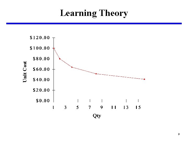
Unit Cost Learning Theory Qty 3

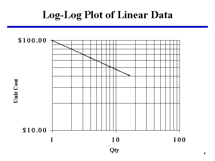
Unit Cost Log-Log Plot of Linear Data Qty 4

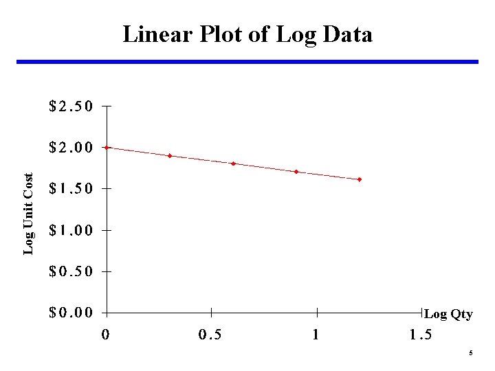
Log Unit Cost Linear Plot of Log Data Log Qty 5

Learning Theory • Two variations: – Cumulative Average Theory – Unit Theory 6

Cumulative Average Theory “If there is learning in the production process, the cumulative average cost of some doubled unit equals the cumulative average cost of the undoubled unit times the slope of the learning curve” • Described by T. P. Wright in 1936 – based on examination of WW I aircraft production costs • Aircraft companies and Do. D were interested in the regular and predictable nature of the reduction in production costs that Wright observed – implied that a fixed amount of labor and facilities would produce greater and greater quantities in successive periods 7

Unit Theory “If there is learning in the production process, the cost of some doubled unit equals the cost of the undoubled unit times the slope of the learning curve” • Credited to J. R. Crawford in 1947 – led a study of WWII airframe production commissioned by USAF to validate learning curve theory 8

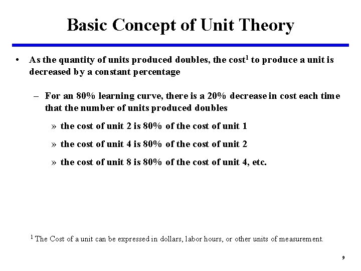
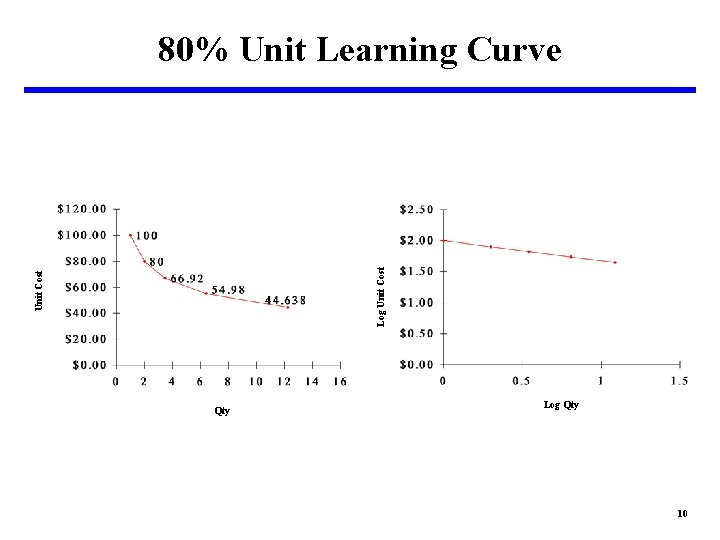
Basic Concept of Unit Theory • As the quantity of units produced doubles, the cost 1 to produce a unit is decreased by a constant percentage – For an 80% learning curve, there is a 20% decrease in cost each time that the number of units produced doubles » the cost of unit 2 is 80% of the cost of unit 1 » the cost of unit 4 is 80% of the cost of unit 2 » the cost of unit 8 is 80% of the cost of unit 4, etc. 1 The Cost of a unit can be expressed in dollars, labor hours, or other units of measurement. 9

Unit Cost Log Unit Cost 80% Unit Learning Curve Qty Log Qty 10

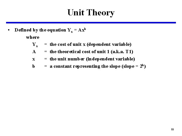
Unit Theory • Defined by the equation Yx = Axb where Yx = the cost of unit x (dependent variable) A = theoretical cost of unit 1 (a. k. a. T 1) x = the unit number (independent variable) b = a constant representing the slope (slope = 2 b) 11

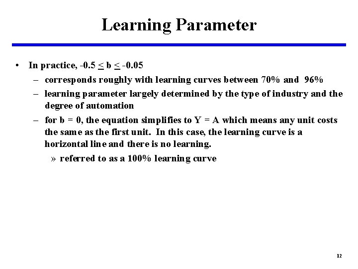
Learning Parameter • In practice, -0. 5 < b < -0. 05 – corresponds roughly with learning curves between 70% and 96% – learning parameter largely determined by the type of industry and the degree of automation – for b = 0, the equation simplifies to Y = A which means any unit costs the same as the first unit. In this case, the learning curve is a horizontal line and there is no learning. » referred to as a 100% learning curve 12

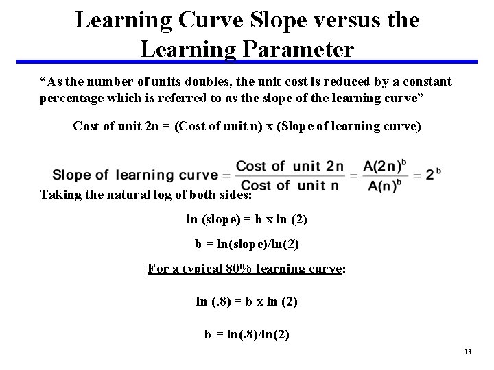
Learning Curve Slope versus the Learning Parameter “As the number of units doubles, the unit cost is reduced by a constant percentage which is referred to as the slope of the learning curve” Cost of unit 2 n = (Cost of unit n) x (Slope of learning curve) Taking the natural log of both sides: ln (slope) = b x ln (2) b = ln(slope)/ln(2) For a typical 80% learning curve: ln (. 8) = b x ln (2) b = ln(. 8)/ln(2) 13

Slope and 1 st Unit Cost • To use a learning curve for a cost estimate, a slope and 1 st unit cost are required – slope may be derived from analogous production situations, industry averages, historical slopes for the same production site, or historical data from previous production quantities – 1 st unit costs may be derived from engineering estimates, CERs, or historical data from previous production quantities 14

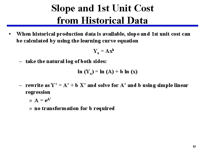
Slope and 1 st Unit Cost from Historical Data • When historical production data is available, slope and 1 st unit cost can be calculated by using the learning curve equation Yx = Axb – take the natural log of both sides: ln (Yx) = ln (A) + b ln (x) – rewrite as Y’ = A’ + b X’ and solve for A’ and b using simple linear regression » A = e. A’ » no transformation for b required 15

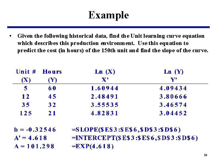
Example • Given the following historical data, find the Unit learning curve equation which describes this production environment. Use this equation to predict the cost (in hours) of the 150 th unit and find the slope of the curve. 16

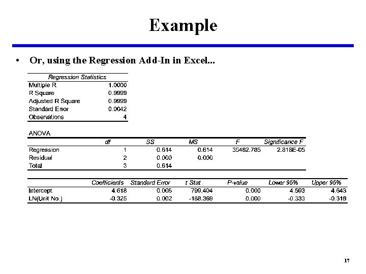
Example • Or, using the Regression Add-In in Excel. . . 17

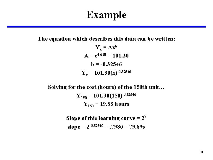
Example The equation which describes this data can be written: Yx = Axb A = e 4. 618 = 101. 30 b = -0. 32546 Yx = 101. 30(x)-0. 32546 Solving for the cost (hours) of the 150 th unit… Y 150 = 101. 30(150)-0. 32546 Y 150 = 19. 83 hours Slope of this learning curve = 2 b slope = 2 -0. 32546 =. 7980 = 79. 8% 18

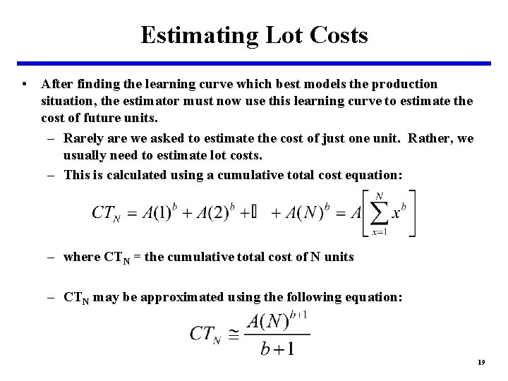
Estimating Lot Costs • After finding the learning curve which best models the production situation, the estimator must now use this learning curve to estimate the cost of future units. – Rarely are we asked to estimate the cost of just one unit. Rather, we usually need to estimate lot costs. – This is calculated using a cumulative total cost equation: – where CTN = the cumulative total cost of N units – CTN may be approximated using the following equation: 19

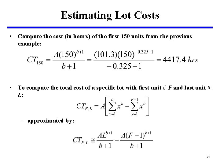
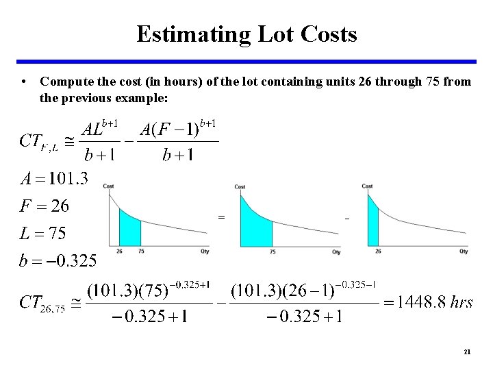
Estimating Lot Costs • Compute the cost (in hours) of the first 150 units from the previous example: • To compute the total cost of a specific lot with first unit # F and last unit # L: – approximated by: 20

Estimating Lot Costs • Compute the cost (in hours) of the lot containing units 26 through 75 from the previous example: = - 21

Fitting a Curve Using Lot Data • Cost data is generally reported for production lots (i. e. , lot cost and units per lot), not individual units – Lot data must be adjusted since learning curve calculations require a unit number and its associated unit cost – Unit number and unit cost for a lot are represented by algebraic lot midpoint (LMP) and average unit cost (AUC) 22

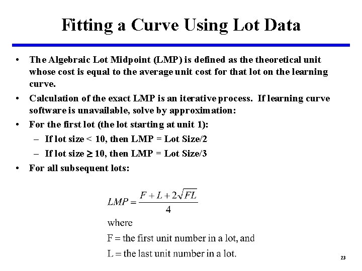
Fitting a Curve Using Lot Data • The Algebraic Lot Midpoint (LMP) is defined as theoretical unit whose cost is equal to the average unit cost for that lot on the learning curve. • Calculation of the exact LMP is an iterative process. If learning curve software is unavailable, solve by approximation: • For the first lot (the lot starting at unit 1): – If lot size < 10, then LMP = Lot Size/2 – If lot size 10, then LMP = Lot Size/3 • For all subsequent lots: 23

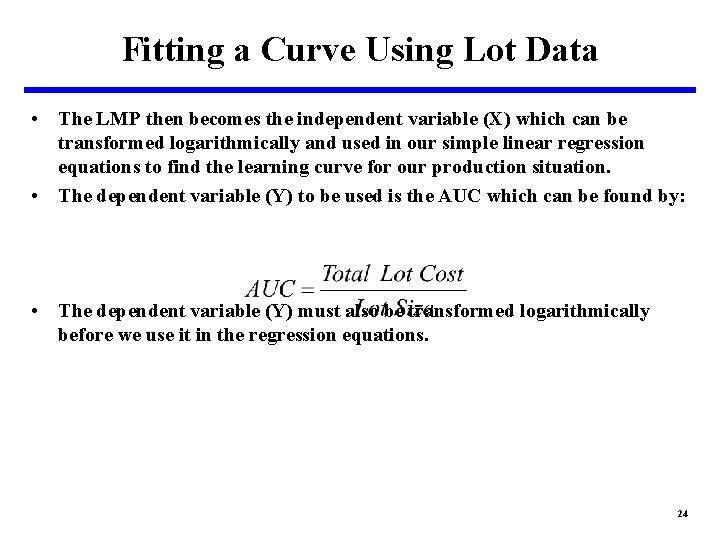
Fitting a Curve Using Lot Data • The LMP then becomes the independent variable (X) which can be transformed logarithmically and used in our simple linear regression equations to find the learning curve for our production situation. • The dependent variable (Y) to be used is the AUC which can be found by: • The dependent variable (Y) must also be transformed logarithmically before we use it in the regression equations. 24

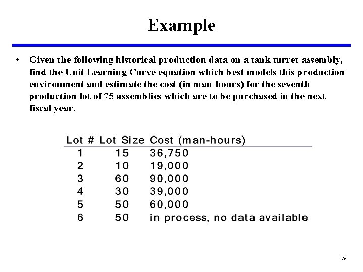
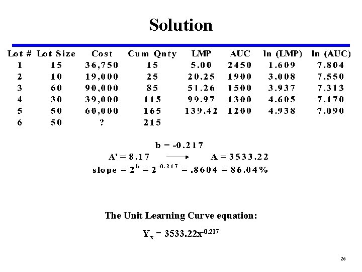
Example • Given the following historical production data on a tank turret assembly, find the Unit Learning Curve equation which best models this production environment and estimate the cost (in man-hours) for the seventh production lot of 75 assemblies which are to be purchased in the next fiscal year. 25

Solution The Unit Learning Curve equation: Yx = 3533. 22 x-0. 217 26

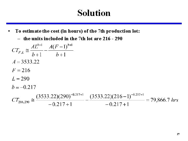
Solution • To estimate the cost (in hours) of the 7 th production lot: – the units included in the 7 th lot are 216 - 290 27

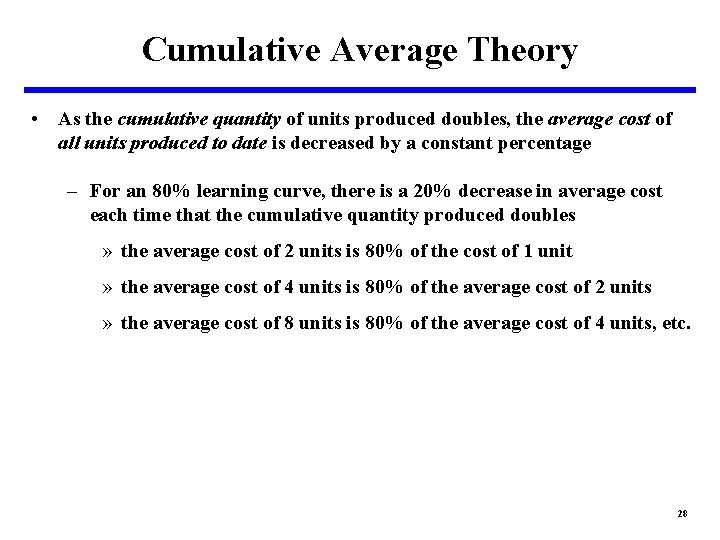
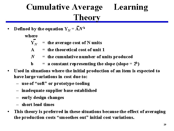
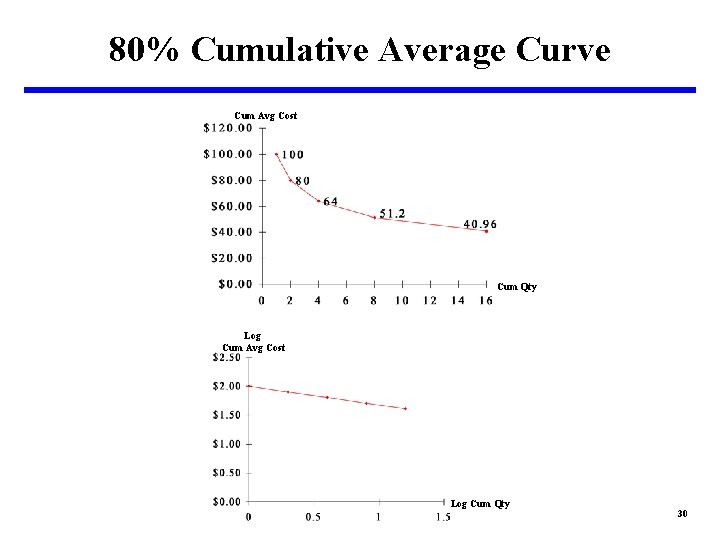
Cumulative Average Theory • As the cumulative quantity of units produced doubles, the average cost of all units produced to date is decreased by a constant percentage – For an 80% learning curve, there is a 20% decrease in average cost each time that the cumulative quantity produced doubles » the average cost of 2 units is 80% of the cost of 1 unit » the average cost of 4 units is 80% of the average cost of 2 units » the average cost of 8 units is 80% of the average cost of 4 units, etc. 28

Cumulative Average Theory Learning • Defined by the equation YN = AN b where YN = the average cost of N units A = theoretical cost of unit 1 N = the cumulative number of units produced b = a constant representing the slope (slope = 2 b) • Used in situations where the initial production of an item is expected to have large variations in cost due to: – use of “soft” or prototype tooling – inadequate supplier base established – early design changes – short lead times • This theory is preferred in these situations because the effect of averaging the production costs “smoothes out” initial cost variations. 29

80% Cumulative Average Curve Cum Avg Cost Cum Qty Log Cum Avg Cost Log Cum Qty 30

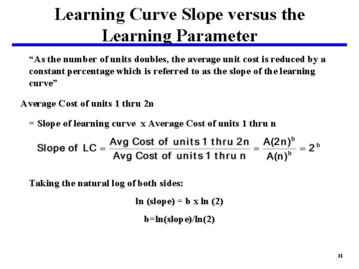
Learning Curve Slope versus the Learning Parameter “As the number of units doubles, the average unit cost is reduced by a constant percentage which is referred to as the slope of the learning curve” Average Cost of units 1 thru 2 n = Slope of learning curve x Average Cost of units 1 thru n Taking the natural log of both sides: ln (slope) = b x ln (2) b=ln(slope)/ln(2) 31

Slope and 1 st Unit Cost • To use a learning curve for a cost estimate, a slope and 1 st unit cost are required – slope may be derived from analogous production situations, industry averages, historical slopes for the same production site, or historical data from previous production quantities – 1 st unit costs may be derived from engineering estimates, CERs, or historical data from previous production quantities 32

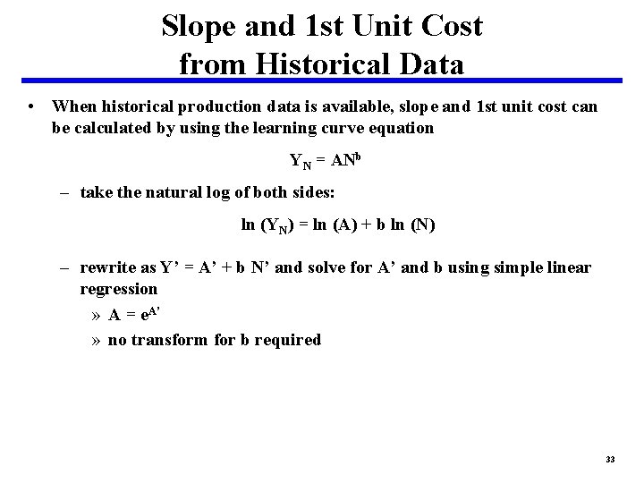
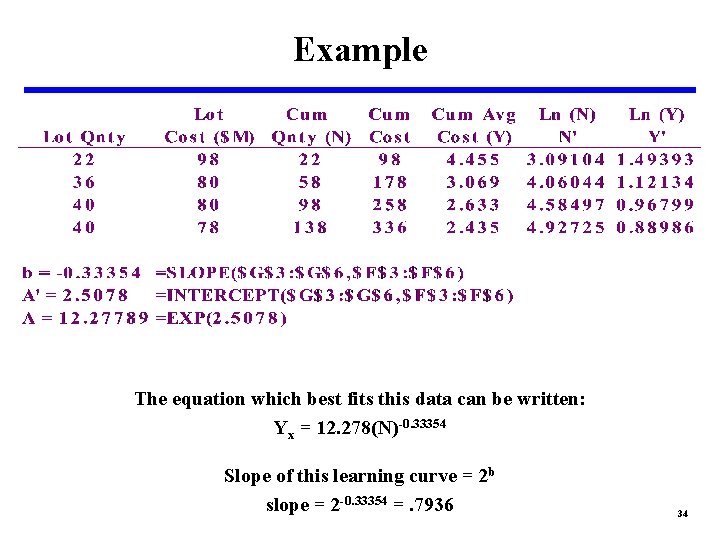
Slope and 1 st Unit Cost from Historical Data • When historical production data is available, slope and 1 st unit cost can be calculated by using the learning curve equation YN = ANb – take the natural log of both sides: ln (YN) = ln (A) + b ln (N) – rewrite as Y’ = A’ + b N’ and solve for A’ and b using simple linear regression » A = e. A’ » no transform for b required 33

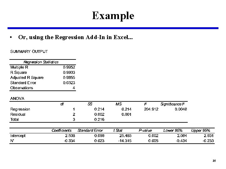
Example The equation which best fits this data can be written: Yx = 12. 278(N)-0. 33354 Slope of this learning curve = 2 b slope = 2 -0. 33354 =. 7936 34

Example • Or, using the Regression Add-In in Excel. . . 35

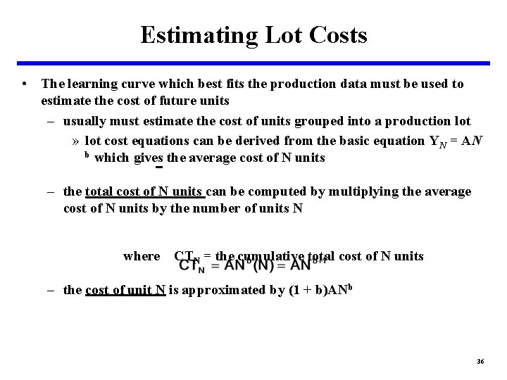
Estimating Lot Costs • The learning curve which best fits the production data must be used to estimate the cost of future units – usually must estimate the cost of units grouped into a production lot » lot cost equations can be derived from the basic equation YN = AN b which gives the average cost of N units – the total cost of N units can be computed by multiplying the average cost of N units by the number of units N where CTN = the cumulative total cost of N units – the cost of unit N is approximated by (1 + b)AN b 36

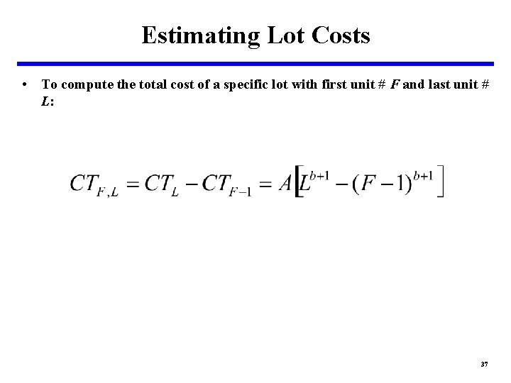
Estimating Lot Costs • To compute the total cost of a specific lot with first unit # F and last unit # L: 37

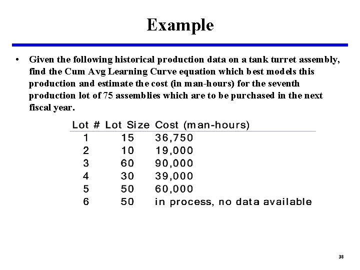
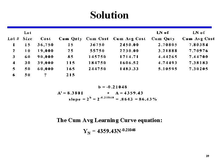
Example • Given the following historical production data on a tank turret assembly, find the Cum Avg Learning Curve equation which best models this production and estimate the cost (in man-hours) for the seventh production lot of 75 assemblies which are to be purchased in the next fiscal year. 38

Solution The Cum Avg Learning Curve equation: YN = 4359. 43 N-0. 21048 39

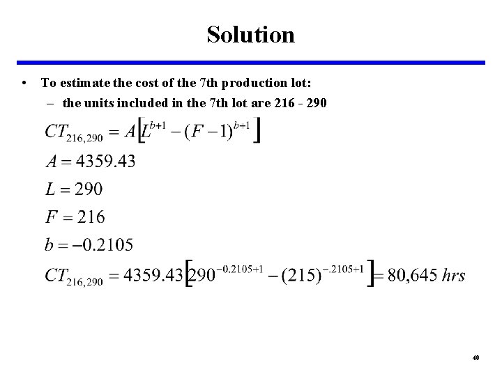
Solution • To estimate the cost of the 7 th production lot: – the units included in the 7 th lot are 216 - 290 40

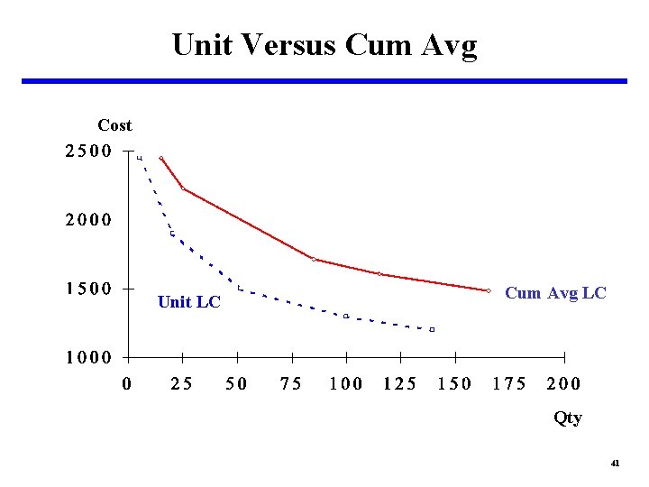
Unit Versus Cum Avg Cost Unit LC Cum Avg LC Qty 41

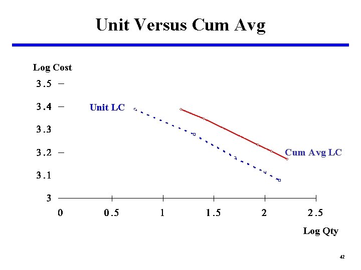
Unit Versus Cum Avg Log Cost Unit LC Cum Avg LC Log Qty 42

Unit versus Cum Avg • Since the Cum Avg curve is based on the average cost of a production quantity rather than the cost of a particular unit, it is less responsive to cost trends than the unit cost curve. – A sizable change in the cost of any unit or lot of units is required before a change is reflected in the Cum Avg curve. » Cum Avg curve is smoother and always has a higher r 2 – Since cost generally decreases, the Unit cost curve will roughly parallel the Cum Avg curve but will always lie below it. » Government negotiator prefers to use Unit cost curve since it is lower and more responsive to recent trends 43

Learning Curve Selection • Type of learning curve to use is an important decision. Factors to consider include: – Analogous Systems » systems which are similar in form, function, or development/production process may provide justification for choosing one theory over another – Industry Standards » certain industries gravitate toward one theory versus another – Historical Experience » some defense contractors have a history of using one theory versus another because it has been shown to best model that contractor’s production process 44

Learning Curve Selection – Expected Production Environment » certain production environments favor one theory over another • Cum Avg: contractor is starting production with prototype tooling, has an inadequate supplier base established, expects early design changes, or is subject to short lead-times • Unit curve: contractor is well prepared to begin production in terms of tooling, suppliers, lead-times, etc. – Statistical Measures » best fit, highest r 2 45

Production Breaks • Production breaks can occur in a program due to funding delays or technical problems. • How much of the learning achieved has been lost (forgotten) due to the break in production? • How will this “lost learning” impact the costs of future production items? • The first question can be answered by using the “Anderlohr Method” for estimating the learning lost. • The second question can then be answered by using the “Retrograde Method” to “reset” the learning curve. 46

Anderlohr Method • To assess the impact on cost of a production break, it is first necessary to quantify how much learning was achieved prior to the break, and then quantify how much of that learning was lost due to the break. • George Anderlohr, a Defense Contract Administration Services (DCAS) employee in the 1960 s, divided the learning lost due to a production break into five categories: – Personnel learning; – Supervisory learning; – Continuity of productivity; – Methods; – Special tooling. 47

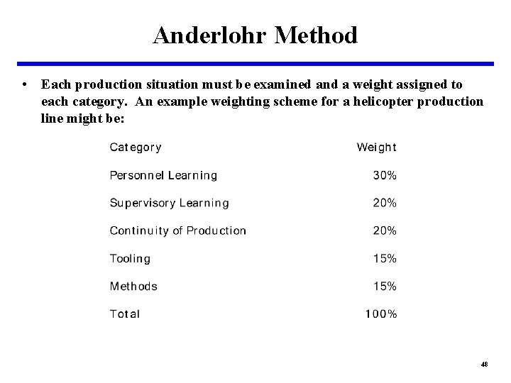
Anderlohr Method • Each production situation must be examined and a weight assigned to each category. An example weighting scheme for a helicopter production line might be: 48

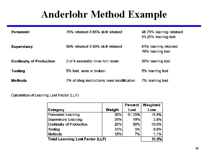
Anderlohr Method • To find the percentage of learning lost (Learning Lost Factor or LLF) we must find the learning lost in each category, and then calculate a weighted average based upon the previous weights. • Example: A contractor who assembles helicopters experiences a sixmonth break in production due to the delayed issuance of a follow-on production contract. The resident Defense Plant Representative Office (DPRO) conducted a survey of the contractor and provided the following information. – During the break in production, the contractor transferred many of his resources to commercial and other defense programs. As a result the following can be expected when production resumes on the helicopter program: 49

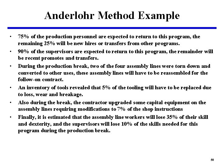
Anderlohr Method Example • • • 75% of the production personnel are expected to return to this program, the remaining 25% will be new hires or transfers from other programs. 90% of the supervisors are expected to return to this program, the remainder will be recent promotes and transfers. During the production break, two of the four assembly lines were torn down and converted to other uses, these assembly lines will have to be reassembled for the follow-on contract. An inventory of tools revealed that 5% of the tooling will have to be replaced due to loss, wear and breakage. Also during the break, the contractor upgraded some capital equipment on the assembly lines requiring modifications to 7% of the shop instructions Finally, it is estimated that the assembly line workers will lose 35% of their skill and dexterity, and the supervisors will lose 10% of the skills needed for this program during the production break. 50

Anderlohr Method Example 51

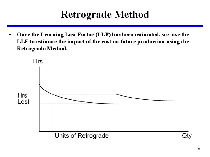
Retrograde Method • Once the Learning Lost Factor (LLF) has been estimated, we use the LLF to estimate the impact of the cost on future production using the Retrograde Method. 52

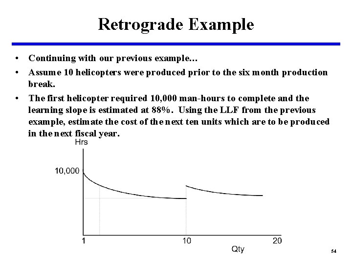
Retrograde Method • The theory is that because you lose hours of learning, the LLF should be applied to the hours of learning that you achieved prior to the break. • The result of the Anderlohr Method gives you the number of hours of learning lost. • These hours can then be added to the cost of the first unit after the break on the original curve to yield an estimate of the cost (in hours) of that unit due to the break in production. • Finally, we can then back up the curve (retrograde) to the point where production costs were equal to our new estimate. 53

Retrograde Example • Continuing with our previous example… • Assume 10 helicopters were produced prior to the six month production break. • The first helicopter required 10, 000 man-hours to complete and the learning slope is estimated at 88%. Using the LLF from the previous example, estimate the cost of the next ten units which are to be produced in the next fiscal year. 54

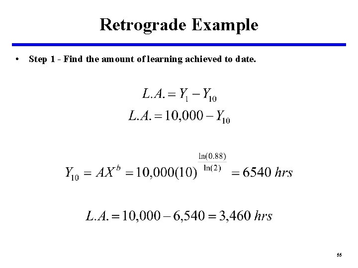
Retrograde Example • Step 1 - Find the amount of learning achieved to date. 55

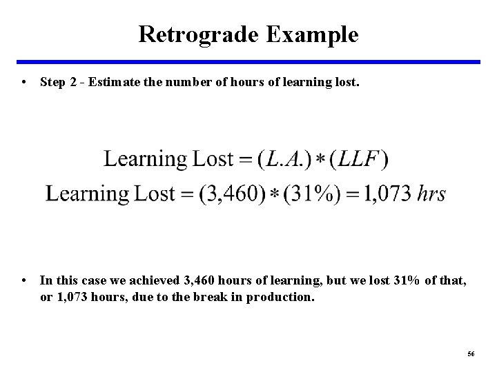
Retrograde Example • Step 2 - Estimate the number of hours of learning lost. • In this case we achieved 3, 460 hours of learning, but we lost 31% of that, or 1, 073 hours, due to the break in production. 56

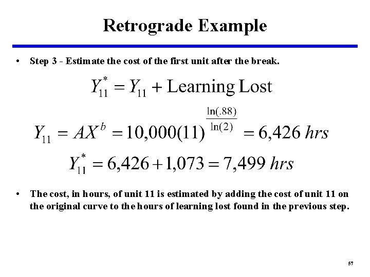
Retrograde Example • Step 3 - Estimate the cost of the first unit after the break. • The cost, in hours, of unit 11 is estimated by adding the cost of unit 11 on the original curve to the hours of learning lost found in the previous step. 57

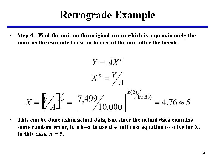
Retrograde Example • Step 4 - Find the unit on the original curve which is approximately the same as the estimated cost, in hours, of the unit after the break. • This can be done using actual data, but since the actual data contains some random error, it is best to use the unit cost equation to solve for X. In this case, X = 5. 58

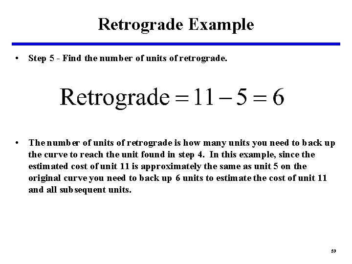
Retrograde Example • Step 5 - Find the number of units of retrograde. • The number of units of retrograde is how many units you need to back up the curve to reach the unit found in step 4. In this example, since the estimated cost of unit 11 is approximately the same as unit 5 on the original curve you need to back up 6 units to estimate the cost of unit 11 and all subsequent units. 59

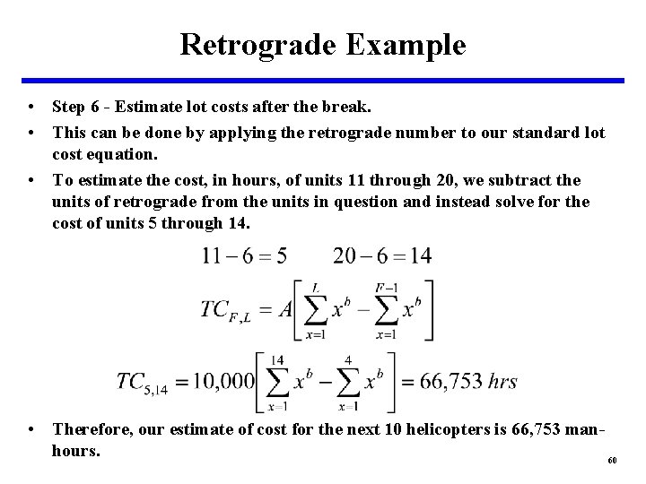
Retrograde Example • Step 6 - Estimate lot costs after the break. • This can be done by applying the retrograde number to our standard lot cost equation. • To estimate the cost, in hours, of units 11 through 20, we subtract the units of retrograde from the units in question and instead solve for the cost of units 5 through 14. • Therefore, our estimate of cost for the next 10 helicopters is 66, 753 manhours. 60

Step-Down Functions • A Step-Down Function is a method of estimating theoretical first unit production cost based upon prototype (development) cost data. • It has been found, in general, that the unit cost of a prototype is more expensive than the first unit cost of a corresponding production model. • The ratio of production first unit cost to prototype average unit cost is known as a Step-Down factor. • An estimate for the Step-Down factor for a given weapon system can be found by examining historical similar weapon systems and developing a cost estimating relationship, with prototype average unit cost as the independent variable. • Once an appropriate CER is developed, it can be used with actual or estimated prototype costs to estimate the first unit production cost. 61

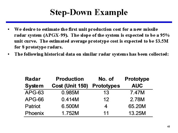
Step-Down Example • We desire to estimate the first unit production cost for a new missile radar system (APGX-99). The slope of the system is expected to be a 95% unit curve. The estimated average prototype cost is expected to be $3. 5 M for 8 prototype radars. • The following historical data on similar radar systems has been collected: 62

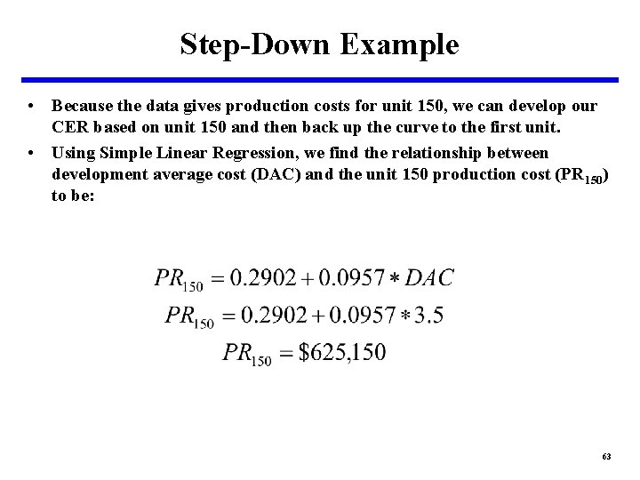
Step-Down Example • Because the data gives production costs for unit 150, we can develop our CER based on unit 150 and then back up the curve to the first unit. • Using Simple Linear Regression, we find the relationship between development average cost (DAC) and the unit 150 production cost (PR 150) to be: 63

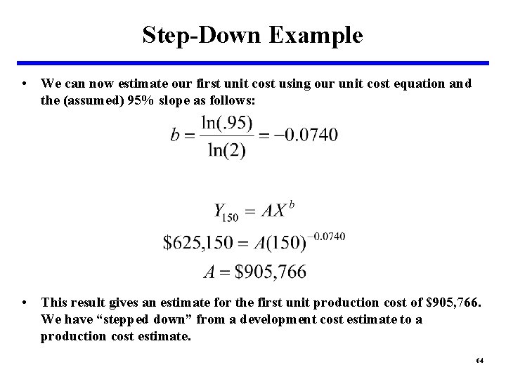
Step-Down Example • We can now estimate our first unit cost using our unit cost equation and the (assumed) 95% slope as follows: • This result gives an estimate for the first unit production cost of $905, 766. We have “stepped down” from a development cost estimate to a production cost estimate. 64

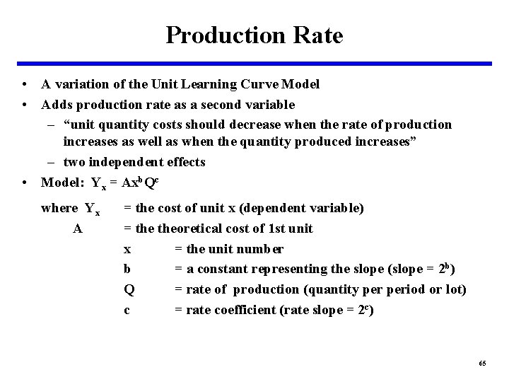
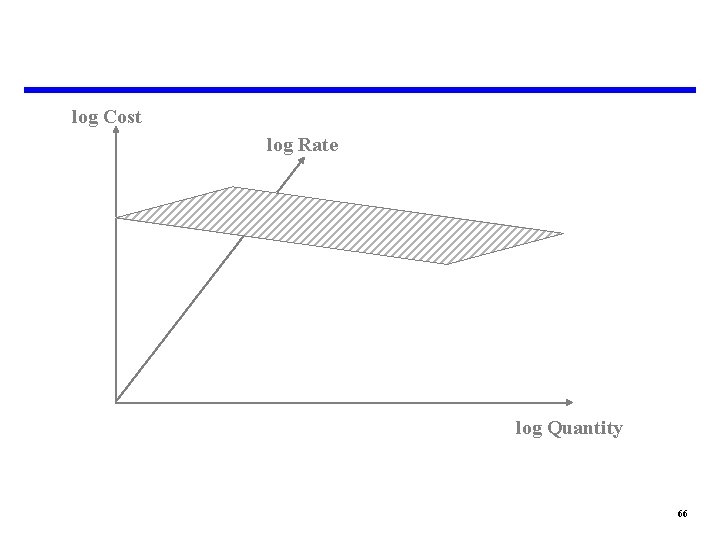
Production Rate • A variation of the Unit Learning Curve Model • Adds production rate as a second variable – “unit quantity costs should decrease when the rate of production increases as well as when the quantity produced increases” – two independent effects • Model: Yx = Axb. Qc where Yx A = the cost of unit x (dependent variable) = theoretical cost of 1 st unit x = the unit number b = a constant representing the slope (slope = 2 b) Q = rate of production (quantity period or lot) c = rate coefficient (rate slope = 2 c) 65

log Cost log Rate log Quantity 66

Rate Model Advantages • It directly models cost reductions which are achieved through economies of scale – quantity discounts received when ordering bulk quantities – reduced ordering and processing costs – reduced shipping, receiving, and inspection costs 67

Rate Model Weaknesses • Appropriate production rate (i. e. , annual, quarterly, monthly) is not always clear • If Q is always increasing, there tends to be a high degree of collinearity between the quantity and rate variables • Always estimates decreasing unit costs for increasing production rates – when a manufacturer’s capacity is exceeded, unit costs generally increase due to costs of overtime, hiring/training new workers, purchase of new capital, etc. 68

When to Consider a Rate Model • Production involves relatively simple components for which lot size is a much greater cost driver than cumulative quantity • When production is taking place well down the learning curve where it flattens out • When there is a major change in production rate 69

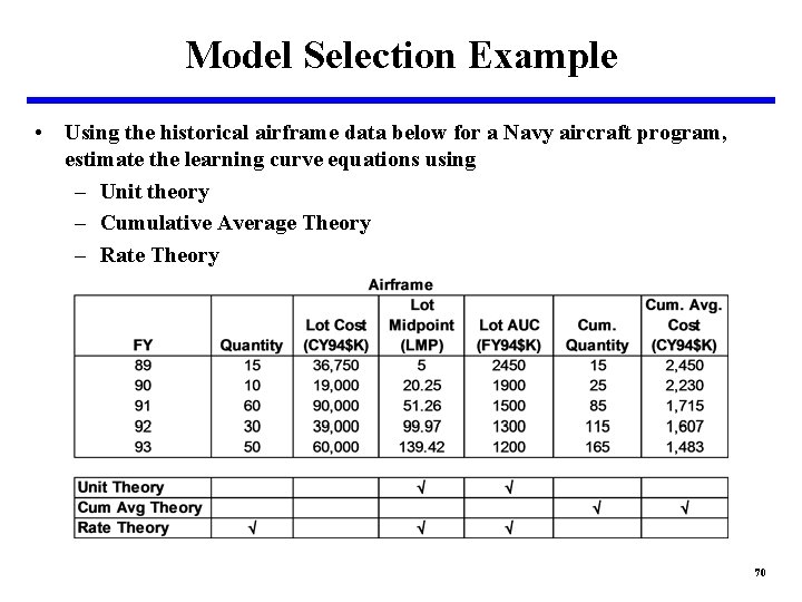
Model Selection Example • Using the historical airframe data below for a Navy aircraft program, estimate the learning curve equations using – Unit theory – Cumulative Average Theory – Rate Theory 70

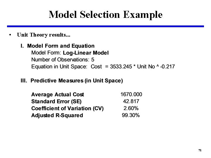
Model Selection Example • Unit Theory results. . . 71

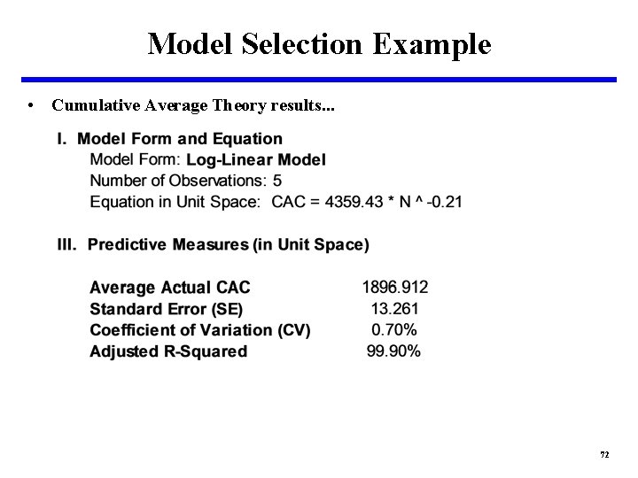
Model Selection Example • Cumulative Average Theory results. . . 72

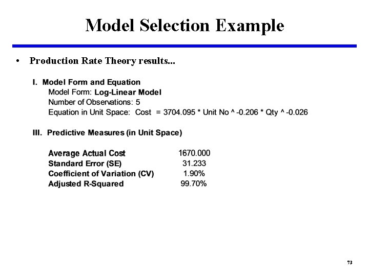
Model Selection Example • Production Rate Theory results. . . 73

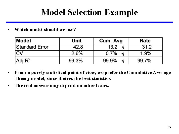
Model Selection Example • Which model should we use? • From a purely statistical point of view, we prefer the Cumulative Average Theory model, since it gives the best statistics. • The real answer may depend on other issues. 74