Electroanalytical chemistry Potentiometry Voltammetry and Polarography Electroanalysis measure

Electroanalytical chemistry Potentiometry, Voltammetry and Polarography

Electroanalysis • measure the variation of an electrical parameter (potential, current, charge, conductivity) and relate this to a chemical parameter (the analyte concentration) • Conductimetry, potentiometry (p. H, ISE), coulometry, voltammetry

Potentiometry the measure of the cell potential to yield chemical information (conc. , activity, charge) Measure difference in potential between two electrodes: reference electrode (E constant) indicator electrode (signal α analyte)

Reference electrodes Ag/Ag. Cl: Ag(s) | Ag. Cl (s) | Cl-(aq) ||. . .

Reference Electrodes SCE: Pt(s) | Hg(l) | Hg 2 Cl 2 (l) | KCl(aq. , sat. ) ||. . .

Indicator Electrodes • Inert: Pt, Au, Carbon. Don’t participate in the reaction. example: SCE || Fe 3+, Fe 2+(aq) | Pt(s) • Certain metallic electrodes: detect their ions (Hg, Cu, Zn, Cd, Ag) example SCE || Ag+(aq) | Ag(s) Ag+ + e- Ag(s) E 0+= 0. 799 V Hg 2 Cl 2 + 2 e 2 Hg(l) + 2 Cl. E-= 0. 241 V E = 0. 799 + 0. 05916 log [Ag+] - 0. 241 V

Ion selective electrodes (ISEs) A difference in the activity of an ion on either side of a selective membrane results in a thermodynamic potential difference being created across that membrane

Membrane Structure(Examples) Glass Membrane Li 2 O, Cs 2 O, La 2 O 3 , Si. O 2 , Ca. O, Ba. O. KM-I pot or KH-Na = 10 -13 Na 2 O (10. 6%), Al 2 O 3(10%), Si. O 2 = (NAS 10. 6 – 10 ) Single Crystal Membrane Mixed Salts Examples on mixed salts For Anions p. H glass electrode KNa-K = 10 -3 Na glass electrode Lanthanum Fluoride La. F 3 doped with Eu, Selective to F- (Ag 2 S + Ag. X) For Anion X, , and (Ag 2 S + MS) For Cations Ag 2 S + Ag. Cl for Cl- Ag 2 S+ Ag. Br for Br- Examples on mixed salts For Cations Ag 2 S + Pb. S for Pb 2+ Liquid Ion Exchanger Calcium didecyl phosphoric acid Ag 2 S + Cu. S for Cu 2+ Ag 2 S + Ag. I for I Ag 2 S + Ag. CN for CN- Ag 2 S + Cd. S for Cd 2+ Ag 2 S + Ni. S for Ni 2+ For Ca 2+

Types of Ion-Selective Electrodes

ISEs

Combination glass p. H Electrode

Proper p. H Calibration • E = constant – constant. 0. 0591 p. H • Meter measures E vs p. H – must calibrate both slope & intercept on meter with buffers • Meter has two controls – calibrate & slope • 1 st use p. H 7. 00 buffer to adjust calibrate knob • 2 nd step is to use any other p. H buffer • Adjust slope/temp control to correct p. H value • This will pivot the calibration line around the isopotential which is set to 7. 00 in all meters Slope/temp control pivots line around isopotential without changing it m. V Calibrate knob raises and lowers the line without changing slope 4 7 p. H

Liquid Membrane Electrodes

Solid State Membrane Electrodes Ag wire Filling solution with fixed [Cl-] and cation that electrode responds to Ag/Ag. Cl Solid state membrane (must be ionic conductor) Solid State Membrane Chemistry Membrane Ion Determined La. F 3 F-, La 3+ Ag. Cl Ag+, Cl. Ag. Br Ag+, Br. Ag. I Ag+, IAg 2 S Ag+, S 2 Ag 2 S + Cu. S Cu 2+ Ag 2 S + Cd. S Cd 2+ Ag 2 S + Pb. S Pb 2+

Nikolsky Equation Selectivity Coefficient, KM-I

Response Time in mins. or seconds needed for the Potential to reach Equilibrium from the point of changing Concn. (t 0 )

Sensitivity of Ion-Selective Electrodes and the Effect of Interferences

Concentration Determination of Ions Using Ion-Selective Electrodes 1 - Direct Potentiometry, (Direct Calibration) The Potential ( E ) of an Ion-Selective Electrode (ISE) is following the concentration of the ion Nernst Equation: E = є ± S/n log a. A In Analytica Chemistry, it is not easy to use activity (a) but to solve this problem, We Consider this relationship: a = µĊ, , where µ is activity coefficient. In order to make a C we must keep µ constant. This can be achieved by Using high concentration Ionic strength of an Inert Electrolyte, or better to Use Total Ionic Strength Adjusting Buffer (TISAB). This is prepared from a high Concentration(such as 1 or 2 M ) mixture of (an Inert Electrolyte such as KNO 3 + a Buffer to adjust p. H + a Ligand to mask metal ion interferences). This solution Is added usually in 1: 1 ratio to all the standards and unknowns. The unknowns Will be determined from the Calibration Curve Which will be plotted now from the modified Nernst Eq. E = є ± S/n log [A]. E is plotted as A function of log[A] According to simplified

2 - Standard Addition, According to This is performed in two ways: a) Single Addition (TISAB is always added) For Simplicity, assume n = 1 and that the analyte is Anion, and E 2 = є - S/n. E 1 = є - S/n E 1 E 2 - E 1 = ΔE = S( = x ) , after Manipulation The final Eq. to find Co will be : E 2

b). Multiple Addition ( Gran’S Plot) • . E 1 = є - S/n . If the left side of this Eq. = F then : : If F = 0 Then Co. Vo = - Cs. Vs which means that F vs Vs is a straight line This is shown in this figure E=є-S F F Vs

3). Potentiometric Titration…. . End Point Detection a). First Derivative, b) Second Derivative… and c) Gran’s Plot You have already studied methods (a and b), we shall now consider ( c ). Gran’s Plot: This method Converts the ( S –shaped)Potentiometric. Titration Curve into a straight line, making the location of (E. P. ) more reliable Let Consider this reaction A+ + BAB Assuming that (A & B ) are Monovalent, the electrode is selective for B- and B- is anion. Accordingly: at the E. P. Co Vo = CA Ve Co = C A V e / V o CB is the Concn. of B at any point remaining in soln. CA VA A Substituting the Value of Co and after necessary Manipulations we obtain Ve E. P B The following Equation : CB or C o Vo

We mentioned before that the Electrode is Selective for B, So it measures B According to Nekolsky Eq. E = є – S log. CB Substituting the Value of CB from the previous Eq. we get: E = є – S log. Then conversion into antilog we obtain the Gran’s Function: Gran’s Plot At the End Point Which means that F = 0 0

Solid state electrodes

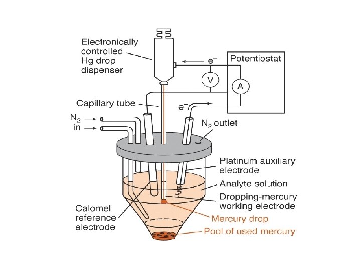
Voltammetry The measurement of variations in current produced by variations of the potential applied to a working electrode polarography: • Heyrovsky (1922): first voltammetry experiments using a dropping mercury working electrode In voltammetry, once the applied potential is sufficiently negative, electron transfer occurs between the electrode and the electroactive species: Cu 2+ + 2 e → Cu(Hg) There are many types of Polarography, but, we shall Study DC Polarography only.

Mass Transport or Mass Transfer • • • Migration – movement of a charged particle in a potential field Diffusion – movement due to a concentration gradient. If electrochemical reaction depletes (or produces) some species at the electrode surface, then a concentration gradient develops and the electroactive species will tend to diffuse from the bulk solution to the electrode (or from the electrode out into the bulk solution) Convection – mass transfer due to stirring. Achieved by some form of mechanical movement of the solution or the electrode i. e. , stir solution, rotate or vibrate electrode Difficult to get perfect reproducibility with stirring, better to move the electrode Convection is considerably more efficient than diffusion or migration = higher currents for a given concentration = greater analytical sensitivity

Diffusion • Movement of mass due to a concentration gradient. Occurs whenever there is chemical change at a surface, e. g. , O R Migration Movement of a charged species due to a potential gradient i. e. Attraction of Opposites Charges Mechanism by which charge passes through electrolyte towards the Electrode Surface Convection Movement of mass due to a natural or mechanical force, such as Stirring or gas bubbling

The mechanism of producing the Diffusion Current (i) i = (n. DFA/ ᵟ)*(C-Co) n = no. of electrons, D = diffusion Coefficient, F = Faraday, A = surface area, ᵟ = Thickness of the diffusion layer, Co mole/L = Cocn. on the drop surface & C mol. /L= Concn. In the bulk of Solution. When the ion concn. On the drop surface becomes zero, Co= 0 and (n. DFA/ ᵟ) is constant = K, then i = id (which is the Limiting Diffusion Current)…. . Thus, the equation above becomes id = K*C But this Equation has been replaced by a more sophisticated Ilkofiҫ Equation as shown below: : Ilkoviç Equation id(max)= 708 n. D 1/2 m 2/3 t 1/6 c Co C id (average)=607 n. D 1/2 m 2/3 t 1/6 c When 708 n. D 1/2 m 2/3 t 1/6 = K, then id = K*C Which is the basis of Quantitative Analysis.

Dropping Mercury Electrode (DME)

The polarogram points a to b I = E/R points b to c electron transfer to the electroactive species. I(reduction) depends on the no. of molecules reduced/s: this rises as a function of E points c to d when E is sufficiently negative, every molecule that reaches the electrode surface is reduced.

Q. . What are the Suitable Electrolyte for the Mixture (1, 2 and 3) and for the Individuals if Present Alone? ? And Why? ?

Effect of Supporting Electrolytes on Polarographic E 1/2 Element 1 MNH 3 + 1 MNH 4+ E 1/2 (V) Values the following Supporting Electrolytes 1 M KCl 7 M H 3 PO 4 1 M Na. OH 1 M KSCN 1 M KCN Cd(II) - 0. 81 - 0. 64 - 0. 71 - 0. 76 - 0. 65 - 1. 18 Co(II) - 1. 29 - 1. 20 - 1. 43 - 1. 06 - 1. 13 Mn(II) - 1. 66 - 1. 51 - 1. 70 - 1. 54 _ Tl(I) - 0. 48 - 0. 63 - 0. 48 - 0. 52 _ Pb(II) _ - 0. 44 - 0. 53 - 0. 76 - 0. 44 - 0. 72 Ni(II) - 1. 10 - 1. 18 _ - 0. 68 - 1. 36 Zn(II) - 1. 35 - 1. 00 - 1. 13 - 1. 53 - 1. 06 _ _

Polarography ( Two Electrodes System)

Dropping Mercury Electrode(DME) Polarography (Three Electrodes System) • Renewable surface • Potential window expanded for reduction (high overpotential for proton reduction at Hg El. )

Polarography

Polarograms E 1/2 = E 0 + RT/n. F log (DR/Do)1/2 (reversible couple) Residual Current Usually D’s are similar so half wave potential is similar to formal potential. Also potential is independent of concentration and can therefore be used as a diagnostic of identity of analytes.

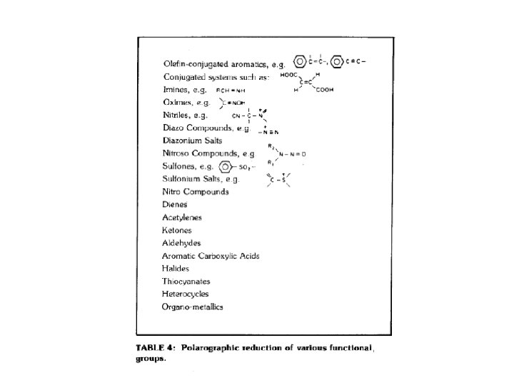
Qualitative and Quantitative Analysis by Polarography Qualitative

Quantitative

Problems in Polarography and Limitations 1 - Dissolved Oxygen O 2 + 2 H 2 O + 2 e = H 2 O 2 + 2 OH • • O 2 + 2 H+ + 2 e = H 2 O 2 + 2 e = 2 OHIn Acidic Medium In Basic Medium H 2 O 2 + 2 H+ + 2 e = 2 H 2 O • • • H 2 O 2 + 2 e = 2 OH- O 2 + 2 H 2 O + 2 e = H 2 O 2 + 2 OH-

id id

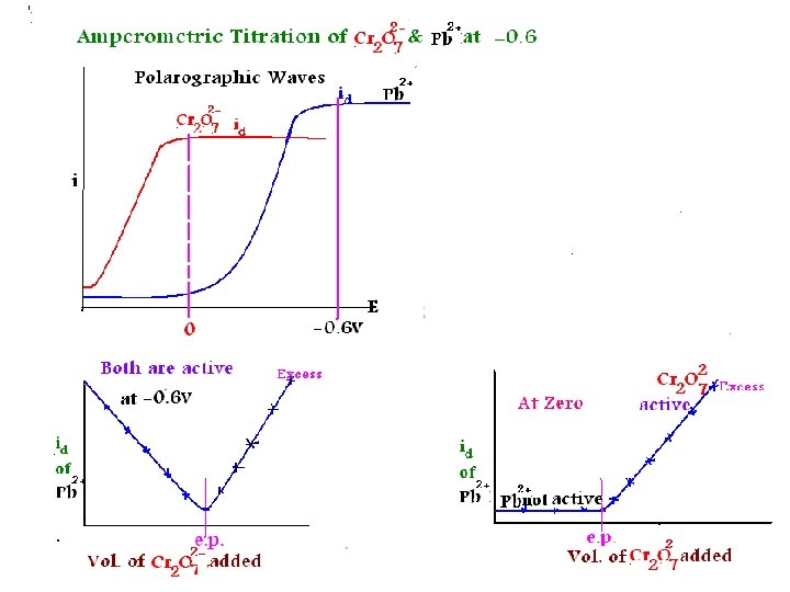
Amperometry

Amperometric Titrations added

COULOMETRY Coulometry is an analytical method for measuring an unknown concentration of an analyte in solution by completely converting the analyte from one oxidation state to another. Coulometry is an absolute measurement similar to gravimetry or titration and requires no chemical standards or calibration.

It is therefore valuable for making absolute concentration determinations of standards. Coulometry uses a constant current source to deliver a measured amount of charge. One mole of electrons is equal to 96, 485 coulombs of charge, and is called a faraday.

Schematic of a coulometric cell

Coulometric Titration Due to concentration polarization it is very difficult to completely oxidize or reduce a chemical species at an electrode. Coulometry is therefore usually done with an intermediate reagent that quantitatively reacts with the analyte. The intermediate reagent is electrochemically generated from an excess of a precursor so that concentration polarization does not occur. An example is the electrochemical oxidation of I- (the precursor) to I 2 (the intermediate reagent). I 2 can then be used to chemically oxidize organic species

The point at which all of the analyte has been converted to the new oxidation state is called the endpoint and is determined by some type of indicator that is also present in the solution. For the coulometric titration of ascorbic acid, starch is used as the indicator. At the endpoint, I 2 remains in solution and binds with the starch to form a dark purple complex. The analyte concentration is calculated from the reaction stoichiometry and the amount of charge that was required to produce enough reagent to react with all of the analyte.

Coulometry and Coulometric Titrations

Coulometric Measurement Two Main procedures are Usually applied for measuring Coulometry: 1 - Using Electronic Coulometry, …. . 2 - Chemical Coulometry (which will be discussed). Chemical Coulometry: Here we discuss the Theory of this Method, which depends on Faraday Law, and water Electrolysis: Total No of moles of One Eq. Wt. of O 2 = One Eq. Wt. of H 2 = Mole O 2 mole H 2 1 F will evolve 1 Eq. Wt. of( O 2 + H 2 ) Thus: 1 F will evolve We must find No of F

Applications of Coulometry 1 -When the Deposition is not possible and 2 - When Deposition is not Successful Fe 2+ = Fe 3+ + e Anodic As. O 3 + H 2 O Cl 3 CC OO- + H+ + 2 e As. O 43 - + 2 H+ + 2 e Anodic Cl 2 CHC OO- + Cl- Cathdic

Examples on Coulometric Titratios 1 - Determination of Sulphide S 2 - E. P. Detection Reagent Generation

Example 2 - 1 - Determination of Sulphide S 2 - - + End Point Detection After switching on The Current (i) will start on Pt Electrode and Br 2 will generate on the Anode On the Pt anode which will Oxidise As. O 33 - to As. O 43 - This Redox reaction Continues and measure Amperometrically Until the First sign of Xss. Br 2 at the End-Point will send a Signal to Switch Off the Reagent Generation. The time t (s) and the Constant Current ( i)amp. Are then Measured and No. of Coulombs(q) is Calculated. q = it…… from here Faraday F is found F = q/96500. Can You Now find the Weight (Wg) of the Analyte Unknown? ? A problem: A constant current of 0. 8 A, was passed through a Cu 2+ solution for 20 min. Find the weight of Deposited Cu on Cathode and Vol. of Librated O 2 on the Anode.

Why Electrons Transfer Reduction E Oxidation EF Eredox E F • Net flow of electrons from M to solute • Ef more negative than Eredox • more cathodic • more reducing • Net flow of electrons from solute to M • Ef more positive than Eredox • more anodic • more oxidizing

Steps in an electron transfer event ØO must be successfully transported from bulk solution (mass transport) ØO must adsorb transiently onto electrode surface (non-faradaic) ØCT must occur between electrode and O (faradaic) ØR must desorb from electrode surface (non-faradaic) ØR must be transported away from electrode surface back into bulk solution (mass transport)

Nernst-Planck Equation Diffusion Migration Convection Ji(x) = flux of species i at distance x from electrode (mole/cm 2 s) Di = diffusion coefficient (cm 2/s) Ci(x)/ x = concentration gradient at distance x from electrode (x)/ x = potential gradient at distance x from electrode (x) = velocity at which species i moves (cm/s)

Diffusion Fick’s 1 st Law I = n. FAJ Solving Fick’s Laws for particular applications like electrochemistry involves establishing Initial Conditions and Boundary Conditions

Simplest Experiment Chronoamperometry

Simulation

Recall-Double layer

Double-Layer charging • Charging/discharging a capacitor upon application of a potential step Itotal = Ic + IF

Working electrode choice • Depends upon potential window desired – Overpotential – Stability of material – Conductivity – contamination

Polarography A = 4 (3 mt/4 d)2/3 = 0. 85(mt)2/3 Density of drop Mass flow rate of drop We can substitute this into Cottrell Equation i(t) = n. FACD 1/2/ 1/2 t 1/2 We also replace D by 7/3 D to account for the compression of the diffusion layer by the expanding drop Giving the Ilkovich Equation: id = 708 n. D 1/2 m 2/3 t 1/6 C I has units of Amps when D is in cm 2 s-1, m is in g/s and t is in seconds. C is in mol/cm 3 This expression gives the current at the end of the drop life. The average current is obtained by integrating the current over this time period iav = 607 n. D 1/2 m 2/3 t 1/6 C

Other types of Polarography • Examples refer to polarography but are applicable to other votammetric methods as well • all attempt to improve signal to noise • usually by removing capacitive currents

Normal Pulse Polarography • current measured at a single instant in the lifetime of each drop. • higher signal because there is more electroactive species around each drop of mercury. • somewhat more sensitive than DC polarography. • data obtained have the same shape as a regular DCP.

NPP advantage • • IL = n. FAD 1/2 c/( tm)1/2 (tm = current sampling t) IL, N. P. /IL, D. C. = (3 t/7 tm)1/2 Predicts that N. P. P. 5 -10 X sensitive than D. C. P.

Differential pulse voltammetry

DPP • current measured twice during the lifetime of each drop difference in current is plotted. • Results in a peak-shaped feature, where the top of the peak corresponds to E 1/2, and the height gives concentration • This shape is the derivative of the regular DC data. • DPP has the advantage of sensitive detection limits and discrimination against background currents. Traditionally, metals in the ppm range can be determined with DPP. • Derivative improves contrast (resolution) between overlapping waves

DPP vs DCP Ep ~ E 1/2 (Ep= E 1/2±DE/2) where DE=pulse amplitude s = exp[(n. F/RT)(DE/2)] Resolution depends on DE W 1/2 = 3. 52 RT/n. F when DE 0 Improved response because charging current is subtracted and adsorptive effects are discriminated against. l. o. d. 10 -8 M

Resolution

Square wave voltammetry

SWV

SWV Response

SWV • advantage of square wave voltammetry is that the entire scan be performed on a single mercury drop in about 10 seconds, as opposed to about 5 minutes for the techniques described previously. SWV saves time, reduces the amount of mercury used per scan by a factor of 100. If used with a prereduction step, detection limits of 1 -10 ppb can be achieved, which rivals graphite furnace AA in sensitivity. • data for SWV similar to DPP • height and width of the wave depends on the exact combination of experimental parameters (i. e. scan rate and pulse height

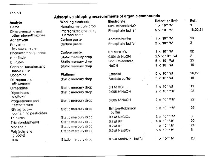
Stripping Voltammetry • Preconcentration technique. 1. Preconcentration or accumulation step. Here the analyte species is collected onto/into the working electrode 2. Measurement step : here a potential waveform is applied to the electrode to remove (strip) the accumulated analyte.

Deposition potential

ASV

ASV or CSV

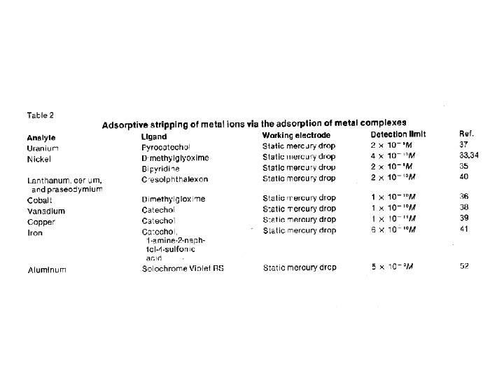
Adsorptive Stripping Voltammetry • Use a chelating ligand that adsorbs to the WE. • Can detect by redox process of metal or ligand.

Multi-Element

Standard Addition

Conductometry and Conductometric Titration

Conductometric Titration If the Ion Concn. = C eq. /L, This means that the Volume that Contains 1 eq. wt = 1000/C So, Ʌ = K. 1000

Conductometric Titration • A Simple Example is a Titration between Stron Acid and Strong Bade • H + X + M + OH In Soln. At any point before E. P. At the E. P After E. P In the Burette M+ , H + Cl- M+ , OHCl- H O + M + X