Econometrics I Professor William Greene Stern School of

Econometrics I Professor William Greene Stern School of Business Department of Economics 14 -/59 Part 14: Generalized Regression

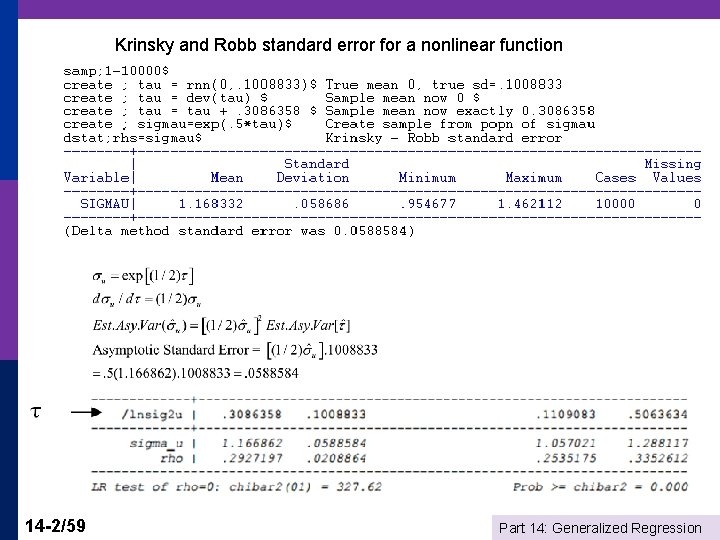
Krinsky and Robb standard error for a nonlinear function 14 -2/59 Part 14: Generalized Regression

Econometrics I Part 14 – Generalized Regression 14 -/59 Part 14: Generalized Regression

Generalized Regression Model Setting: The classical linear model assumes that E[ ] = Var[ ] = 2 I. That is, observations are uncorrelated and all are drawn from a distribution with the same variance. The generalized regression (GR) model allows the variances to differ across observations and allows correlation across observations. 14 -4/59 Part 14: Generalized Regression

Generalized Regression Model The generalized regression model: y = X + , E[ |X] = 0, Var[ |X] = 2. Regressors are well behaved. Trace = n. This is a ‘normalization. ’ Mimics tr( 2 I) = n 2. Needed since p Leading Cases p n n n 14 -5/59 Simple heteroscedasticity Autocorrelation Panel data and heterogeneity more generally. SUR Models for Production and Cost VAR models in Macroeconomics and Finance Part 14: Generalized Regression

Implications of GR Assumptions p p 14 -6/59 The assumption that Var[ ] = 2 I is used to derive the result Var[b] = 2(X X)-1. If it is not true, then the use of s 2(X X)-1 to estimate Var[b] is inappropriate. The assumption was also used to derive the t and F test statistics, so they must be revised as well. Least squares gives each observation a weight of 1/n. But, if the variances are not equal, then some observations are more informative than others. Least squares is based on simple sums, so the information that one observation might provide about another is never used. Part 14: Generalized Regression

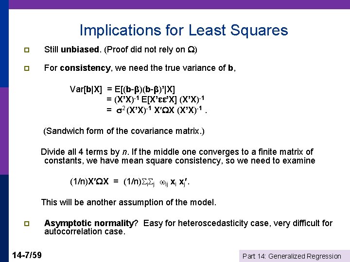
Implications for Least Squares p Still unbiased. (Proof did not rely on ) p For consistency, we need the true variance of b, Var[b|X] = E[(b-β)’|X] = (X’X)-1 E[X’εε’X] (X’X)-1 = 2 (X’X)-1 X X (X’X)-1. (Sandwich form of the covariance matrix. ) Divide all 4 terms by n. If the middle one converges to a finite matrix of constants, we have mean square consistency, so we need to examine (1/n)X X = (1/n) i j ij xi xj. This will be another assumption of the model. p 14 -7/59 Asymptotic normality? Easy for heteroscedasticity case, very difficult for autocorrelation case. Part 14: Generalized Regression

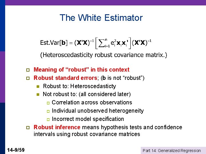
Robust Covariance Matrix Robust estimation: Generality p How to estimate Var[b|X] = (X’X)-1 X ( 2 )X(X’X)-1 for the LS b? p The distinction between estimating 2 an n n matrix and estimating the K K matrix 2 X X = 2 i j ij xi xj p NOTE…… VVVIRs for modern applied econometrics. p n n 14 -8/59 The White estimator Newey-West estimator. Part 14: Generalized Regression

The White Estimator p p p 14 -9/59 Meaning of “robust” in this context Robust standard errors; (b is not “robust”) n Robust to: Heteroscedasticty n Not robust to: (all considered later) p Correlation across observations p Individual unobserved heterogeneity p Incorrect model specification Robust inference means hypothesis tests and confidence intervals using robust covariance matrices Part 14: Generalized Regression

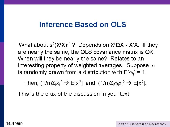
Inference Based on OLS What about s 2(X X)-1 ? Depends on X X - X X. If they are nearly the same, the OLS covariance matrix is OK. When will they be nearly the same? Relates to an interesting property of weighted averages. Suppose i is randomly drawn from a distribution with E[ i] = 1. Then, (1/n) ixi 2 E[x 2] and (1/n) i ixi 2 E[x 2]. This is the crux of the discussion in your text. 14 -10/59 Part 14: Generalized Regression

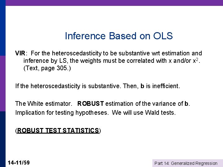
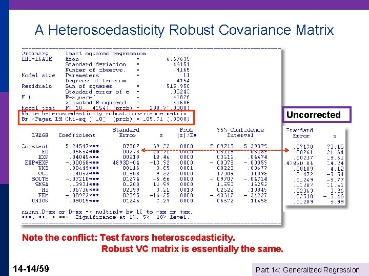
Inference Based on OLS VIR: For the heteroscedasticity to be substantive wrt estimation and inference by LS, the weights must be correlated with x and/or x 2. (Text, page 305. ) If the heteroscedasticity is substantive. Then, b is inefficient. The White estimator. ROBUST estimation of the variance of b. Implication for testing hypotheses. We will use Wald tests. (ROBUST TEST STATISTICS) 14 -11/59 Part 14: Generalized Regression

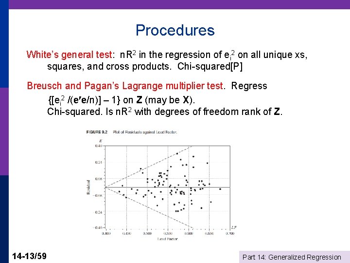
Finding Heteroscedasticity The central issue is whether E[ 2] = 2 i is related to the xs or their squares in the model. Suggests an obvious strategy. Use residuals to estimate disturbances and look for relationships between ei 2 and xi and/or xi 2. For example, regressions of squared residuals on xs and their squares. 14 -12/59 Part 14: Generalized Regression

Procedures White’s general test: n. R 2 in the regression of ei 2 on all unique xs, squares, and cross products. Chi-squared[P] Breusch and Pagan’s Lagrange multiplier test. Regress {[ei 2 /(e e/n)] – 1} on Z (may be X). Chi-squared. Is n. R 2 with degrees of freedom rank of Z. 14 -13/59 Part 14: Generalized Regression

A Heteroscedasticity Robust Covariance Matrix Uncorrected Note the conflict: Test favors heteroscedasticity. Robust VC matrix is essentially the same. 14 -14/59 Part 14: Generalized Regression

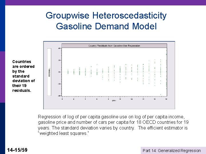
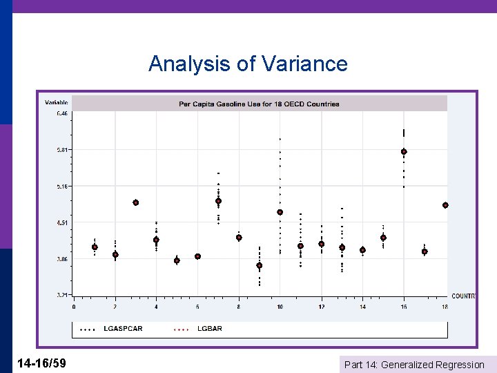
Groupwise Heteroscedasticity Gasoline Demand Model Countries are ordered by the standard deviation of their 19 residuals. Regression of log of per capita gasoline use on log of per capita income, gasoline price and number of cars per capita for 18 OECD countries for 19 years. The standard deviation varies by country. The efficient estimator is “weighted least squares. ” 14 -15/59 Part 14: Generalized Regression

Analysis of Variance 14 -16/59 Part 14: Generalized Regression

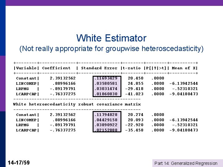
White Estimator (Not really appropriate for groupwise heteroscedasticity) +--------------+--------+--------+-----+ |Variable| Coefficient | Standard Error |t-ratio |P[|T|>t]| Mean of X| +--------------+--------+--------+-----+ Constant| 2. 39132562. 11693429 20. 450. 0000 LINCOMEP|. 88996166. 03580581 24. 855. 0000 -6. 13942544 LRPMG | -. 89179791. 03031474 -29. 418. 0000 -. 52310321 LCARPCAP| -. 76337275. 01860830 -41. 023. 0000 -9. 04180473 ------------------------White heteroscedasticity robust covariance matrix ------------------------Constant| 2. 39132562. 11794828 20. 274. 0000 LINCOMEP|. 88996166. 04429158 20. 093. 0000 -6. 13942544 LRPMG | -. 89179791. 03890922 -22. 920. 0000 -. 52310321 LCARPCAP| -. 76337275. 02152888 -35. 458. 0000 -9. 04180473 14 -17/59 Part 14: Generalized Regression

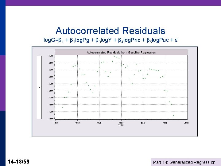
Autocorrelated Residuals log. G=β 1 + β 2 log. Pg + β 3 log. Y + β 4 log. Pnc + β 5 log. Puc + ε 14 -18/59 Part 14: Generalized Regression

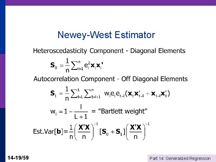
Newey-West Estimator 14 -19/59 Part 14: Generalized Regression

Newey-West Estimate ----+------------------------------Variable| Coefficient Standard Error t-ratio P[|T|>t] Mean of X ----+------------------------------Constant| -21. 2111***. 75322 -28. 160. 0000 LP| -. 02121. 04377 -. 485. 6303 3. 72930 LY| 1. 09587***. 07771 14. 102. 0000 9. 67215 LPNC| -. 37361**. 15707 -2. 379. 0215 4. 38037 LPUC|. 02003. 10330. 194. 8471 4. 10545 --------+------------------------------------------------------------Variable| Coefficient Standard Error t-ratio P[|T|>t] Mean of X Robust VC Newey-West, Periods = 10 ----+------------------------------Constant| -21. 2111*** 1. 33095 -15. 937. 0000 LP| -. 02121. 06119 -. 347. 7305 3. 72930 LY| 1. 09587***. 14234 7. 699. 0000 9. 67215 LPNC| -. 37361**. 16615 -2. 249. 0293 4. 38037 LPUC|. 02003. 14176. 141. 8882 4. 10545 ----+------------------------------- 14 -20/59 Part 14: Generalized Regression

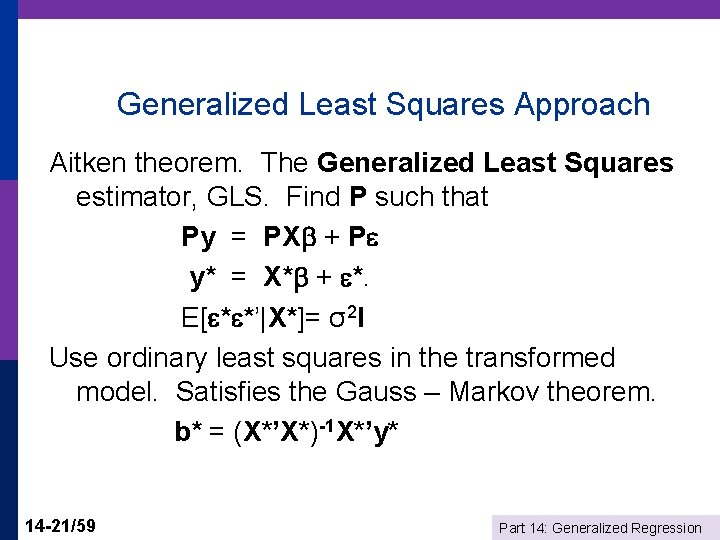
Generalized Least Squares Approach Aitken theorem. The Generalized Least Squares estimator, GLS. Find P such that Py = PX + P y* = X* + *. E[ * *’|X*]= σ2 I Use ordinary least squares in the transformed model. Satisfies the Gauss – Markov theorem. b* = (X*’X*)-1 X*’y* 14 -21/59 Part 14: Generalized Regression

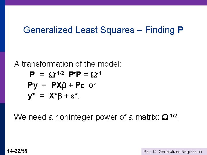
Generalized Least Squares – Finding P A transformation of the model: P = -1/2. P P = -1 Py = PX + P or y* = X* + *. We need a noninteger power of a matrix: -1/2. 14 -22/59 Part 14: Generalized Regression

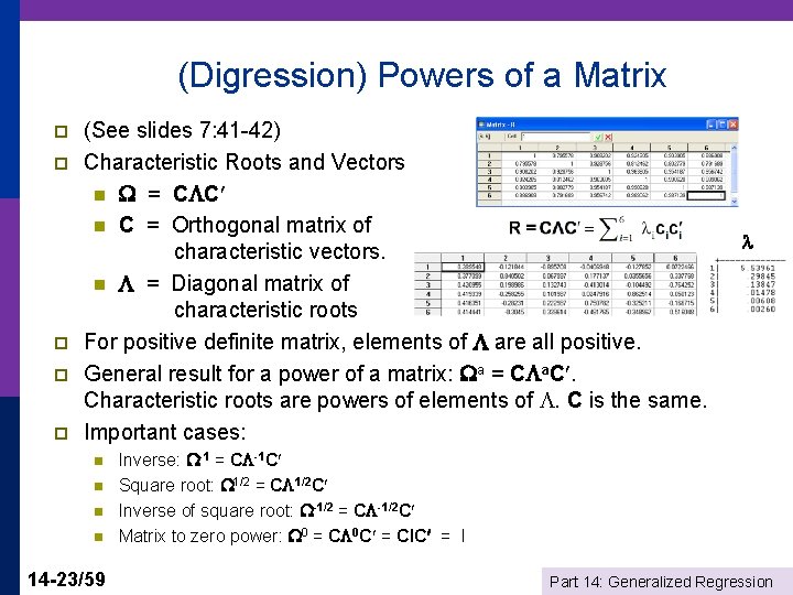
(Digression) Powers of a Matrix p p p (See slides 7: 41 -42) Characteristic Roots and Vectors n = C C n C = Orthogonal matrix of characteristic vectors. n = Diagonal matrix of characteristic roots For positive definite matrix, elements of are all positive. General result for a power of a matrix: a = C a. C. Characteristic roots are powers of elements of . C is the same. Important cases: n n 14 -23/59 Inverse: -1 = C -1 C Square root: 1/2 = C 1/2 C Inverse of square root: -1/2 = C -1/2 C Matrix to zero power: 0 = C 0 C = CIC = I Part 14: Generalized Regression

Generalized Least Squares – Finding P (Using powers of the matrix) E[ * *’|X*] = PE[ | X*]P = PE[ |X]P = σ2 P P = σ2 -1/2 = σ2 0 = σ2 I 14 -24/59 Part 14: Generalized Regression

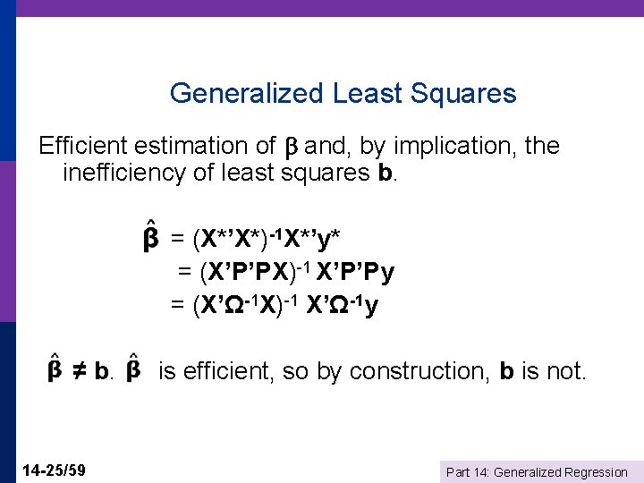
Generalized Least Squares Efficient estimation of and, by implication, the inefficiency of least squares b. = (X*’X*)-1 X*’y* = (X’P’PX)-1 X’P’Py = (X’Ω-1 X)-1 X’Ω-1 y ≠ b. is efficient, so by construction, b is not. 14 -25/59 Part 14: Generalized Regression

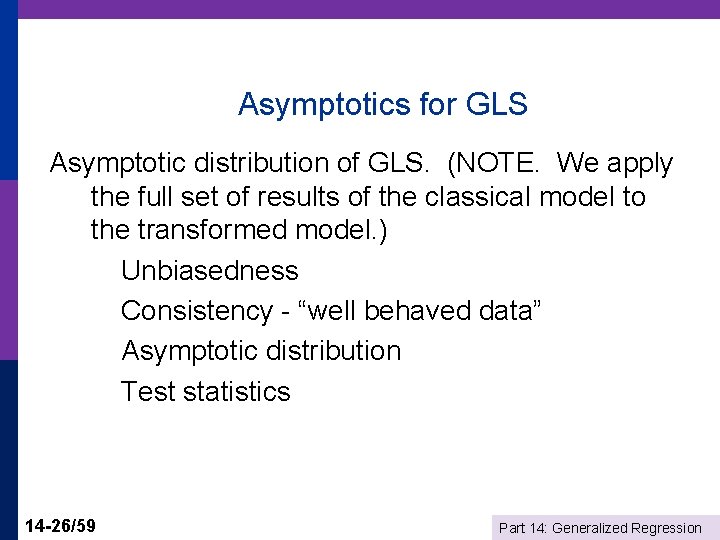
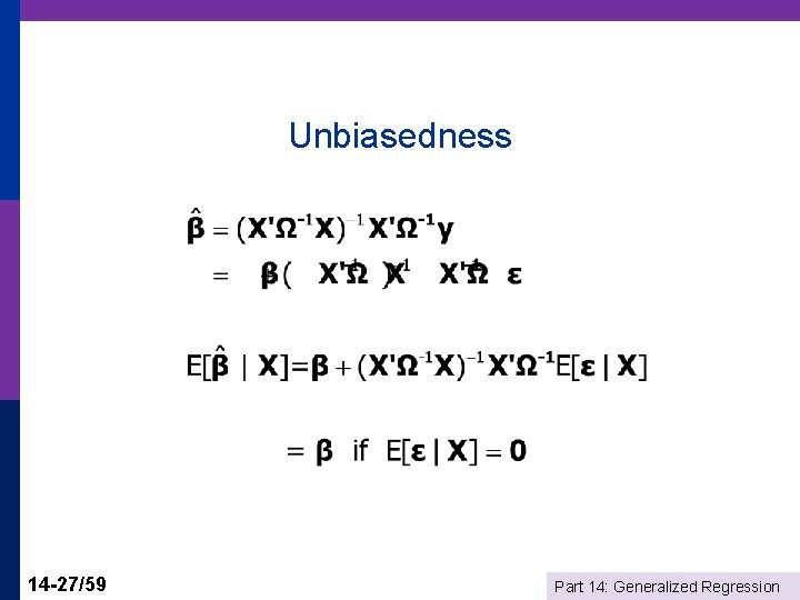
Asymptotics for GLS Asymptotic distribution of GLS. (NOTE. We apply the full set of results of the classical model to the transformed model. ) Unbiasedness Consistency - “well behaved data” Asymptotic distribution Test statistics 14 -26/59 Part 14: Generalized Regression

Unbiasedness 14 -27/59 Part 14: Generalized Regression

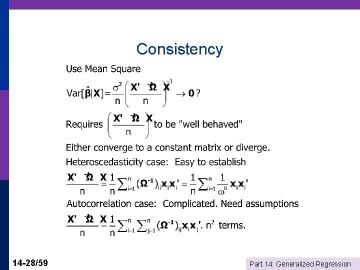
Consistency 14 -28/59 Part 14: Generalized Regression

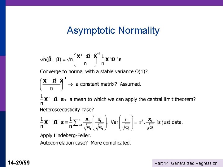
Asymptotic Normality 14 -29/59 Part 14: Generalized Regression

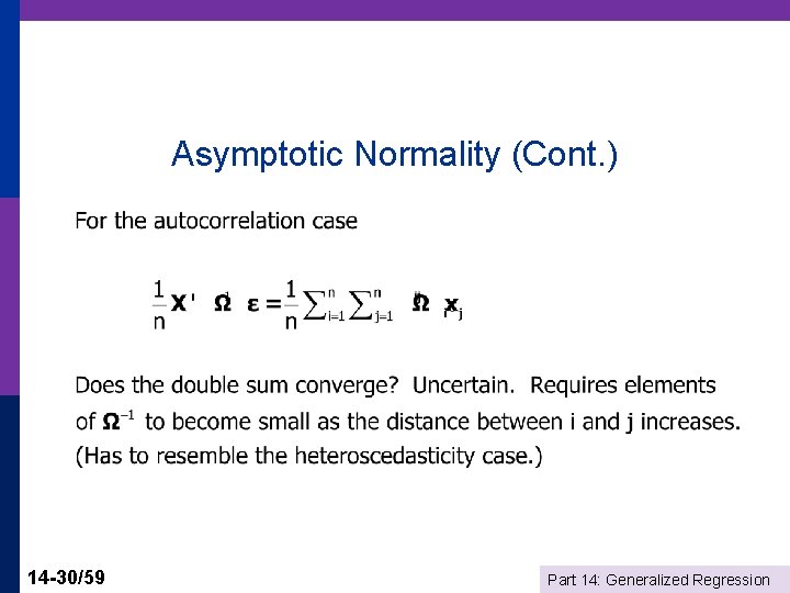
Asymptotic Normality (Cont. ) 14 -30/59 Part 14: Generalized Regression

Test Statistics (Assuming Known Ω) p p p 14 -31/59 With known Ω, apply all familiar results to the transformed model: With normality, t and F statistics apply to least squares based on Py and PX With asymptotic normality, use Wald statistics and the chi-squared distribution, still based on the transformed model. Part 14: Generalized Regression

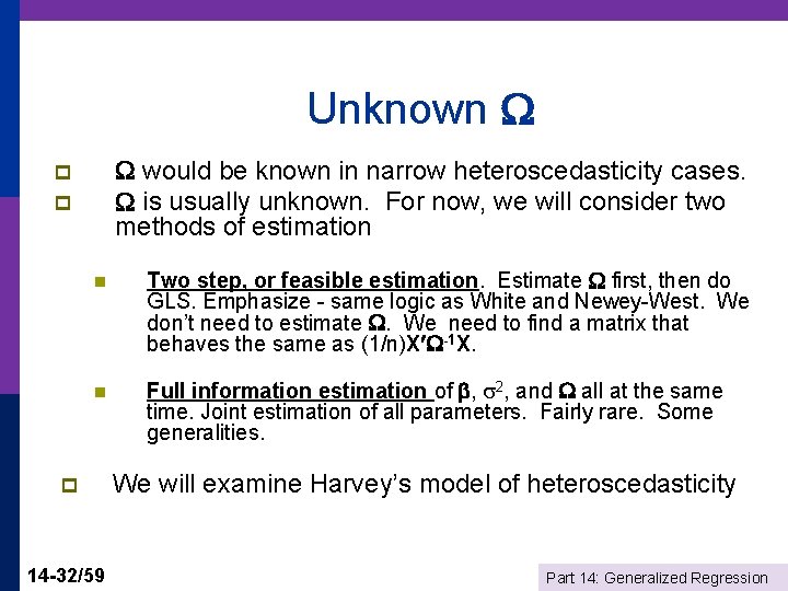
Unknown would be known in narrow heteroscedasticity cases. is usually unknown. For now, we will consider two methods of estimation p p n Two step, or feasible estimation. Estimate first, then do GLS. Emphasize - same logic as White and Newey-West. We don’t need to estimate . We need to find a matrix that behaves the same as (1/n)X -1 X. n Full information estimation of , 2, and all at the same time. Joint estimation of all parameters. Fairly rare. Some generalities. p 14 -32/59 We will examine Harvey’s model of heteroscedasticity Part 14: Generalized Regression

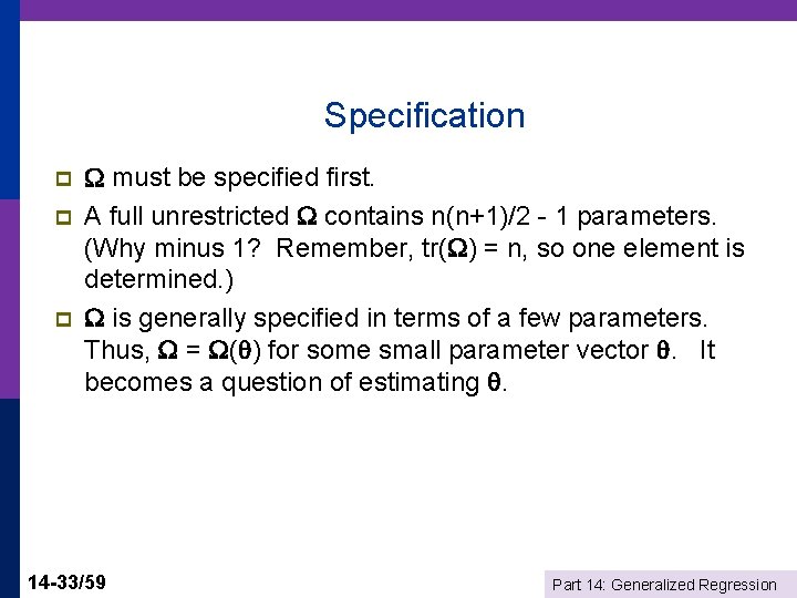
Specification p p p must be specified first. A full unrestricted contains n(n+1)/2 - 1 parameters. (Why minus 1? Remember, tr( ) = n, so one element is determined. ) is generally specified in terms of a few parameters. Thus, = ( ) for some small parameter vector . It becomes a question of estimating . 14 -33/59 Part 14: Generalized Regression

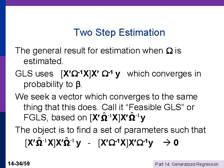
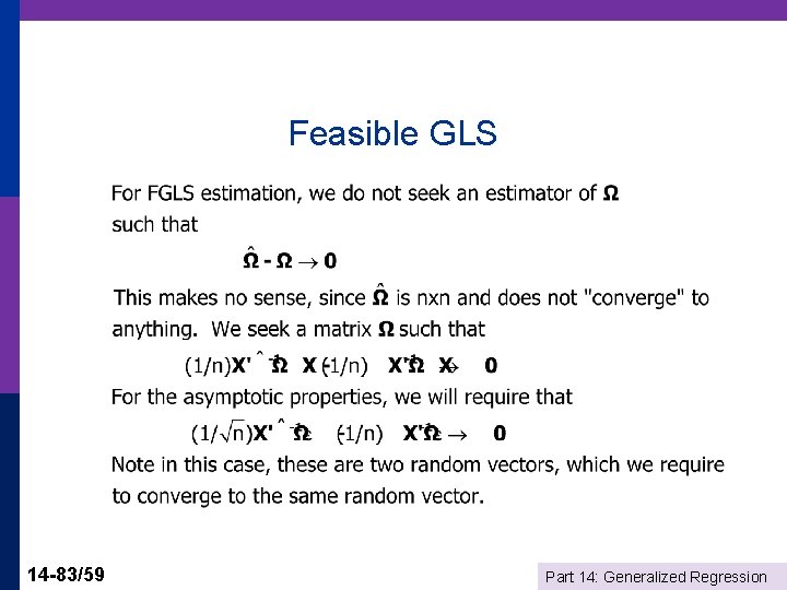
Two Step Estimation The general result for estimation when is estimated. GLS uses [X -1 X]X -1 y which converges in probability to . We seek a vector which converges to the same thing that this does. Call it “Feasible GLS” or FGLS, based on [X X]X y The object is to find a set of parameters such that [X X]X y - [X -1 X]X -1 y 0 14 -34/59 Part 14: Generalized Regression

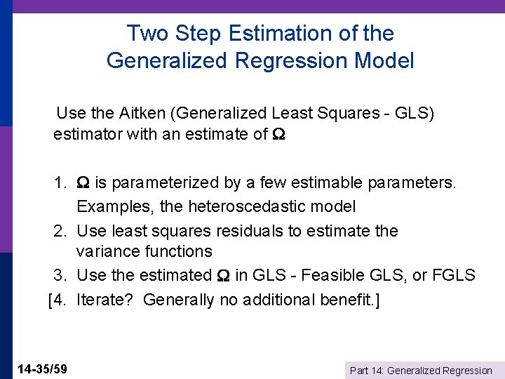
Two Step Estimation of the Generalized Regression Model Use the Aitken (Generalized Least Squares - GLS) estimator with an estimate of 1. is parameterized by a few estimable parameters. Examples, the heteroscedastic model 2. Use least squares residuals to estimate the variance functions 3. Use the estimated in GLS - Feasible GLS, or FGLS [4. Iterate? Generally no additional benefit. ] 14 -35/59 Part 14: Generalized Regression

FGLS vs. Full GLS VVIR (Theorem 9. 5) To achieve full efficiency, we do not need an efficient estimate of the parameters in , only a consistent one. 14 -36/59 Part 14: Generalized Regression

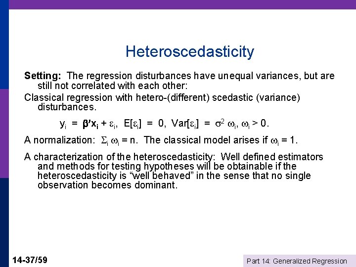
Heteroscedasticity Setting: The regression disturbances have unequal variances, but are still not correlated with each other: Classical regression with hetero-(different) scedastic (variance) disturbances. yi = xi + i, E[ i] = 0, Var[ i] = 2 i, i > 0. A normalization: i i = n. The classical model arises if i = 1. A characterization of the heteroscedasticity: Well defined estimators and methods for testing hypotheses will be obtainable if the heteroscedasticity is “well behaved” in the sense that no single observation becomes dominant. 14 -37/59 Part 14: Generalized Regression

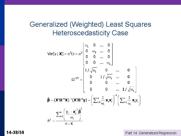
Generalized (Weighted) Least Squares Heteroscedasticity Case 14 -38/59 Part 14: Generalized Regression

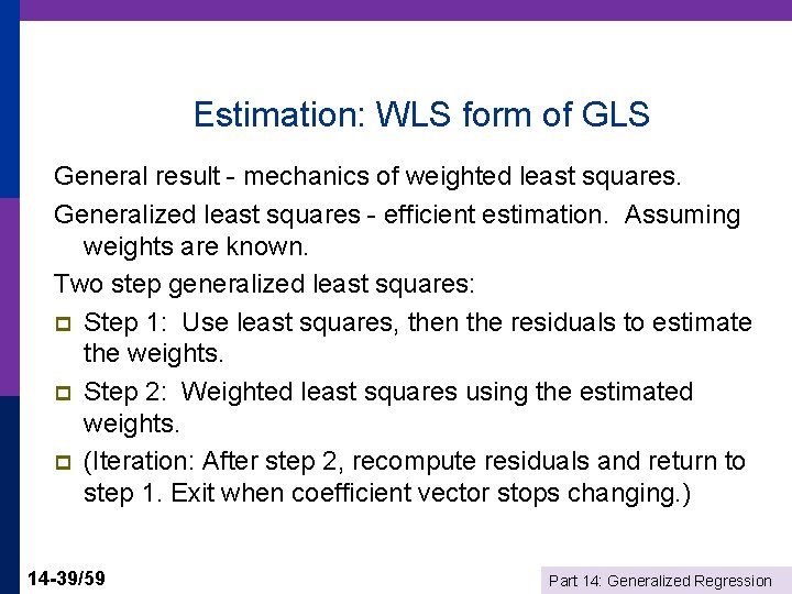
Estimation: WLS form of GLS General result - mechanics of weighted least squares. Generalized least squares - efficient estimation. Assuming weights are known. Two step generalized least squares: p Step 1: Use least squares, then the residuals to estimate the weights. p Step 2: Weighted least squares using the estimated weights. p (Iteration: After step 2, recompute residuals and return to step 1. Exit when coefficient vector stops changing. ) 14 -39/59 Part 14: Generalized Regression

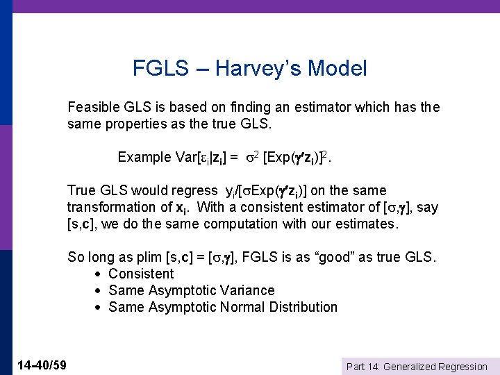
FGLS – Harvey’s Model Feasible GLS is based on finding an estimator which has the same properties as the true GLS. Example Var[ i|zi] = 2 [Exp( zi)]2. True GLS would regress yi/[ Exp( zi)] on the same transformation of xi. With a consistent estimator of [ , ], say [s, c], we do the same computation with our estimates. So long as plim [s, c] = [ , ], FGLS is as “good” as true GLS. Consistent Same Asymptotic Variance Same Asymptotic Normal Distribution 14 -40/59 Part 14: Generalized Regression

Harvey’s Model of Heteroscedasticity Var[ i | X] = 2 exp( zi) p Cov[ i, j | X] = 0 e. g. : zi = firm size e. g. : zi = a set of dummy variables (e. g. , countries) (The groupwise heteroscedasticity model. ) p [ 2 ] = diagonal [exp( + zi)], = log( 2) p 14 -41/59 Part 14: Generalized Regression

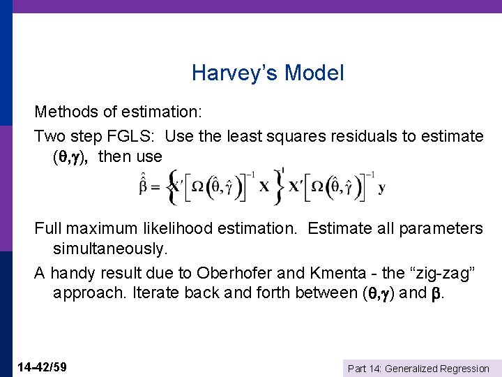
Harvey’s Model Methods of estimation: Two step FGLS: Use the least squares residuals to estimate ( , ), then use Full maximum likelihood estimation. Estimate all parameters simultaneously. A handy result due to Oberhofer and Kmenta - the “zig-zag” approach. Iterate back and forth between ( , ) and . 14 -42/59 Part 14: Generalized Regression

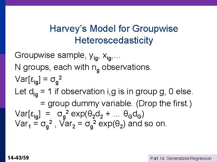
Harvey’s Model for Groupwise Heteroscedasticity Groupwise sample, yig, xig, … N groups, each with ng observations. Var[εig] = σg 2 Let dig = 1 if observation i, g is in group g, 0 else. = group dummy variable. (Drop the first. ) Var[εig] = σg 2 exp(θ 2 d 2 + … θGd. G) Var 1 = σg 2 , Var 2 = σg 2 exp(θ 2) and so on. 14 -43/59 Part 14: Generalized Regression

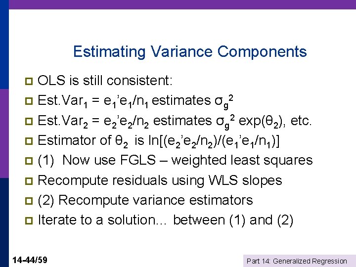
Estimating Variance Components OLS is still consistent: p Est. Var 1 = e 1’e 1/n 1 estimates σg 2 p Est. Var 2 = e 2’e 2/n 2 estimates σg 2 exp(θ 2), etc. p Estimator of θ 2 is ln[(e 2’e 2/n 2)/(e 1’e 1/n 1)] p (1) Now use FGLS – weighted least squares p Recompute residuals using WLS slopes p (2) Recompute variance estimators p Iterate to a solution… between (1) and (2) p 14 -44/59 Part 14: Generalized Regression

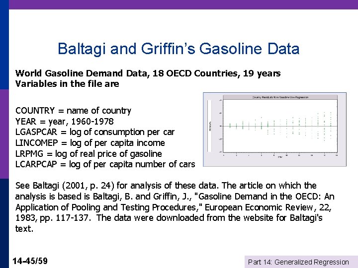
Baltagi and Griffin’s Gasoline Data World Gasoline Demand Data, 18 OECD Countries, 19 years Variables in the file are COUNTRY = name of country YEAR = year, 1960 -1978 LGASPCAR = log of consumption per car LINCOMEP = log of per capita income LRPMG = log of real price of gasoline LCARPCAP = log of per capita number of cars See Baltagi (2001, p. 24) for analysis of these data. The article on which the analysis is based is Baltagi, B. and Griffin, J. , "Gasoline Demand in the OECD: An Application of Pooling and Testing Procedures, " European Economic Review, 22, 1983, pp. 117 -137. The data were downloaded from the website for Baltagi's text. 14 -45/59 Part 14: Generalized Regression

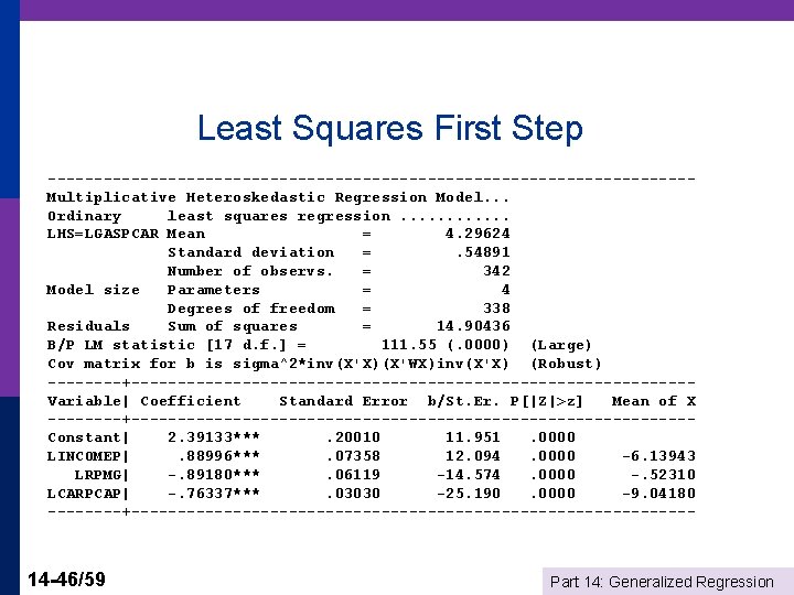
Least Squares First Step -----------------------------------Multiplicative Heteroskedastic Regression Model. . . Ordinary least squares regression. . . LHS=LGASPCAR Mean = 4. 29624 Standard deviation =. 54891 Number of observs. = 342 Model size Parameters = 4 Degrees of freedom = 338 Residuals Sum of squares = 14. 90436 B/P LM statistic [17 d. f. ] = 111. 55 (. 0000) (Large) Cov matrix for b is sigma^2*inv(X'X)(X'WX)inv(X'X) (Robust) ----+------------------------------Variable| Coefficient Standard Error b/St. Er. P[|Z|>z] Mean of X ----+------------------------------Constant| 2. 39133***. 20010 11. 951. 0000 LINCOMEP|. 88996***. 07358 12. 094. 0000 -6. 13943 LRPMG| -. 89180***. 06119 -14. 574. 0000 -. 52310 LCARPCAP| -. 76337***. 03030 -25. 190. 0000 -9. 04180 ----+------------------------------- 14 -46/59 Part 14: Generalized Regression

Variance Estimates = ln[e(i)’e(i)/T] Sigma| D 1| D 2| D 3| D 4| D 5| D 6| D 7| D 8| D 9| D 10| D 11| D 12| D 13| D 14| D 15| D 16| D 17| 14 -47/59 . 48196*** -2. 60677*** -1. 52919**. 47152 -3. 15102*** -3. 26236*** -. 09099 -1. 88962***. 60559 -1. 56624** -1. 53284** -2. 62835*** -2. 23638*** -. 77641 -1. 27341* -. 57948 -1. 81723** -2. 93529*** . 12281. 72073. 72073 3. 924 -3. 617 -2. 122. 654 -4. 372 -4. 526 -. 126 -2. 622. 840 -2. 173 -2. 127 -3. 647 -3. 103 -1. 077 -1. 767 -. 804 -2. 521 -4. 073 . 0001. 0003. 0339. 5130. 0000. 8995. 0087. 4008. 0298. 0334. 0003. 0019. 2814. 0773. 4214. 0117. 0000 . 05556. 05556 Part 14: Generalized Regression

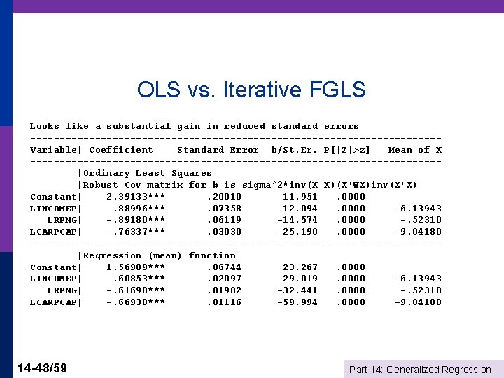
OLS vs. Iterative FGLS Looks like a substantial gain in reduced standard errors ----+------------------------------Variable| Coefficient Standard Error b/St. Er. P[|Z|>z] Mean of X ----+------------------------------|Ordinary Least Squares |Robust Cov matrix for b is sigma^2*inv(X'X)(X'WX)inv(X'X) Constant| 2. 39133***. 20010 11. 951. 0000 LINCOMEP|. 88996***. 07358 12. 094. 0000 -6. 13943 LRPMG| -. 89180***. 06119 -14. 574. 0000 -. 52310 LCARPCAP| -. 76337***. 03030 -25. 190. 0000 -9. 04180 ----+------------------------------|Regression (mean) function Constant| 1. 56909***. 06744 23. 267. 0000 LINCOMEP|. 60853***. 02097 29. 019. 0000 -6. 13943 LRPMG| -. 61698***. 01902 -32. 441. 0000 -. 52310 LCARPCAP| -. 66938***. 01116 -59. 994. 0000 -9. 04180 14 -48/59 Part 14: Generalized Regression

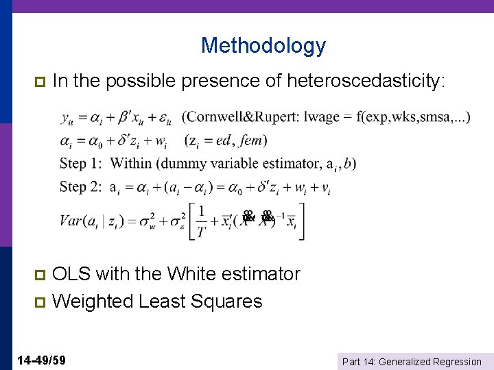
Methodology p In the possible presence of heteroscedasticity: OLS with the White estimator p Weighted Least Squares p 14 -49/59 Part 14: Generalized Regression

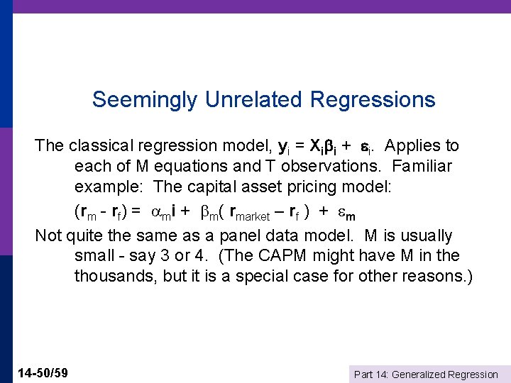
Seemingly Unrelated Regressions The classical regression model, yi = Xi i + i. Applies to each of M equations and T observations. Familiar example: The capital asset pricing model: (rm - rf) = mi + m( rmarket – rf ) + m Not quite the same as a panel data model. M is usually small - say 3 or 4. (The CAPM might have M in the thousands, but it is a special case for other reasons. ) 14 -50/59 Part 14: Generalized Regression

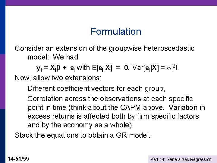
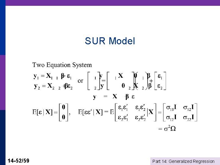
Formulation Consider an extension of the groupwise heteroscedastic model: We had yi = Xi + i with E[ i|X] = 0, Var[ i|X] = i 2 I. Now, allow two extensions: Different coefficient vectors for each group, Correlation across the observations at each specific point in time (think about the CAPM above. Variation in excess returns is affected both by firm specific factors and by the economy as a whole). Stack the equations to obtain a GR model. 14 -51/59 Part 14: Generalized Regression

SUR Model 14 -52/59 Part 14: Generalized Regression

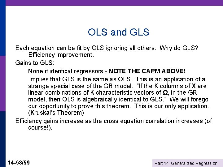
OLS and GLS Each equation can be fit by OLS ignoring all others. Why do GLS? Efficiency improvement. Gains to GLS: None if identical regressors - NOTE THE CAPM ABOVE! Implies that GLS is the same as OLS. This is an application of a strange special case of the GR model. “If the K columns of X are linear combinations of K characteristic vectors of , in the GR model, then OLS is algebraically identical to GLS. ” We will forego our opportunity to prove this theorem. This is our only application. (Kruskal’s Theorem) Efficiency gains increase as the cross equation correlation increases (of course!). 14 -53/59 Part 14: Generalized Regression

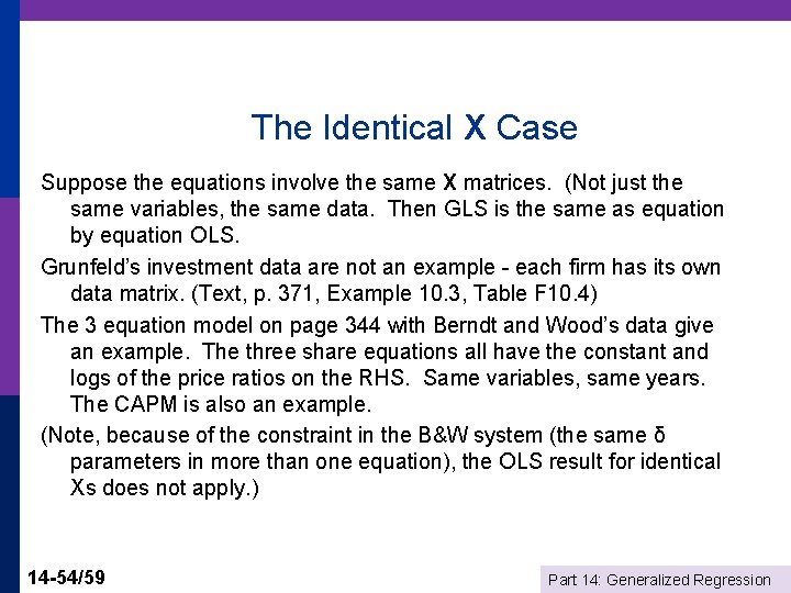
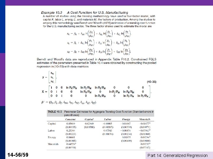
The Identical X Case Suppose the equations involve the same X matrices. (Not just the same variables, the same data. Then GLS is the same as equation by equation OLS. Grunfeld’s investment data are not an example - each firm has its own data matrix. (Text, p. 371, Example 10. 3, Table F 10. 4) The 3 equation model on page 344 with Berndt and Wood’s data give an example. The three share equations all have the constant and logs of the price ratios on the RHS. Same variables, same years. The CAPM is also an example. (Note, because of the constraint in the B&W system (the same δ parameters in more than one equation), the OLS result for identical Xs does not apply. ) 14 -54/59 Part 14: Generalized Regression

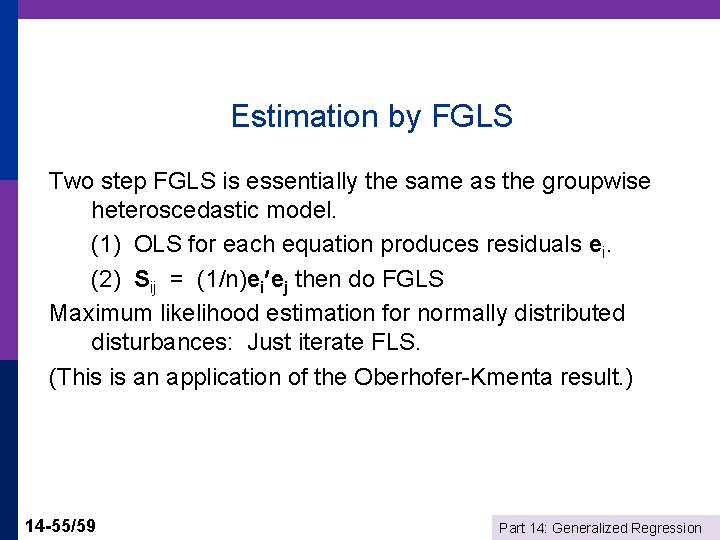
Estimation by FGLS Two step FGLS is essentially the same as the groupwise heteroscedastic model. (1) OLS for each equation produces residuals ei. (2) Sij = (1/n)ei ej then do FGLS Maximum likelihood estimation for normally distributed disturbances: Just iterate FLS. (This is an application of the Oberhofer-Kmenta result. ) 14 -55/59 Part 14: Generalized Regression

14 -56/59 Part 14: Generalized Regression

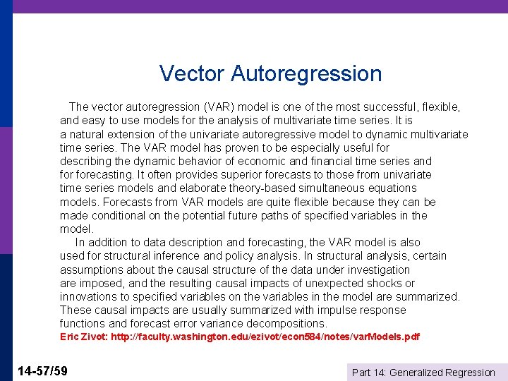
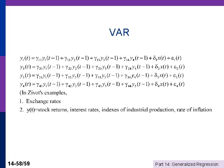
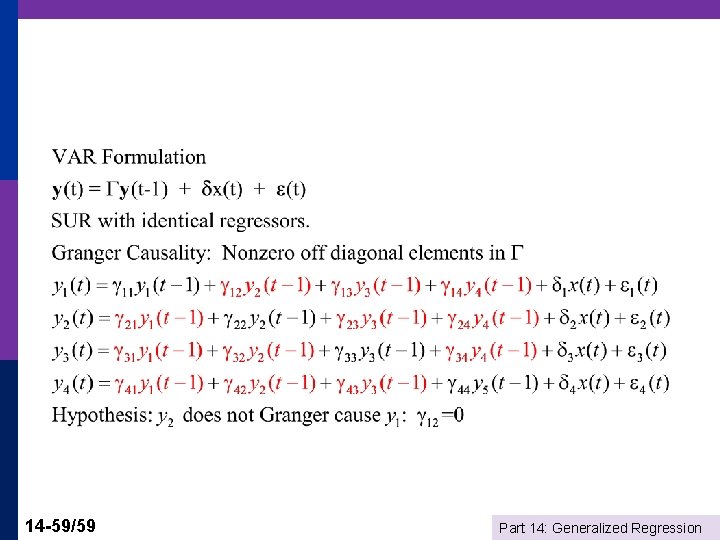
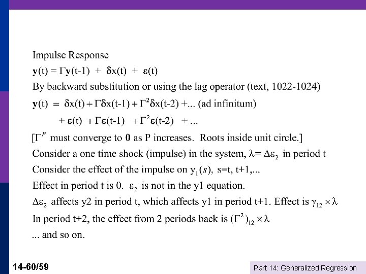
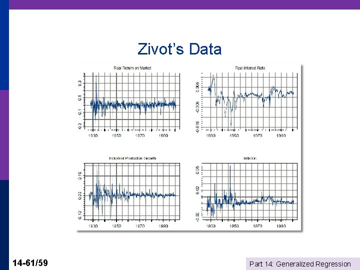
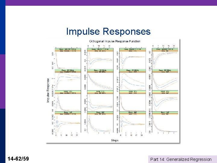
Vector Autoregression The vector autoregression (VAR) model is one of the most successful, flexible, and easy to use models for the analysis of multivariate time series. It is a natural extension of the univariate autoregressive model to dynamic multivariate time series. The VAR model has proven to be especially useful for describing the dynamic behavior of economic and financial time series and forecasting. It often provides superior forecasts to those from univariate time series models and elaborate theory-based simultaneous equations models. Forecasts from VAR models are quite flexible because they can be made conditional on the potential future paths of specified variables in the model. In addition to data description and forecasting, the VAR model is also used for structural inference and policy analysis. In structural analysis, certain assumptions about the causal structure of the data under investigation are imposed, and the resulting causal impacts of unexpected shocks or innovations to specified variables on the variables in the model are summarized. These causal impacts are usually summarized with impulse response functions and forecast error variance decompositions. Eric Zivot: http: //faculty. washington. edu/ezivot/econ 584/notes/var. Models. pdf 14 -57/59 Part 14: Generalized Regression

VAR 14 -58/59 Part 14: Generalized Regression

14 -59/59 Part 14: Generalized Regression

14 -60/59 Part 14: Generalized Regression

Zivot’s Data 14 -61/59 Part 14: Generalized Regression

Impulse Responses 14 -62/59 Part 14: Generalized Regression

Appendix: Autocorrelation in Time Series 14 -63/59 Part 14: Generalized Regression

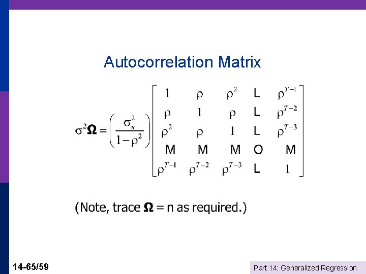
Autocorrelation The analysis of “autocorrelation” in the narrow sense of correlation of the disturbances across time largely parallels the discussions we’ve already done for the GR model in general and for heteroscedasticity in particular. One difference is that the relatively crisp results for the model of heteroscedasticity are replaced with relatively fuzzy, somewhat imprecise results here. The reason is that it is much more difficult to characterize meaningfully “well behaved” data in a time series context. Thus, for example, in contrast to the sharp result that produces the White robust estimator, theory underlying the Newey-West robust estimator is somewhat ambiguous in its requirement of a bland statement about “how far one must go back in time until correlation becomes unimportant. ” 14 -64/59 Part 14: Generalized Regression

Autocorrelation Matrix 14 -65/59 Part 14: Generalized Regression

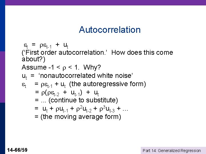
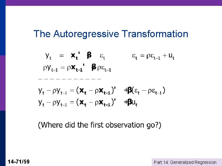
Autocorrelation t = t-1 + ut (‘First order autocorrelation. ’ How does this come about? ) Assume -1 < < 1. Why? ut = ‘nonautocorrelated white noise’ t = t-1 + ut (the autoregressive form) = ( t-2 + ut-1) + ut =. . . (continue to substitute) = ut + ut-1 + 2 ut-2 + 3 ut-3 +. . . = (the moving average form) 14 -66/59 Part 14: Generalized Regression

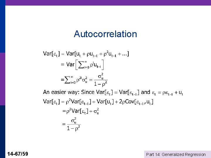
Autocorrelation 14 -67/59 Part 14: Generalized Regression

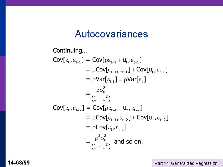
Autocovariances 14 -68/59 Part 14: Generalized Regression

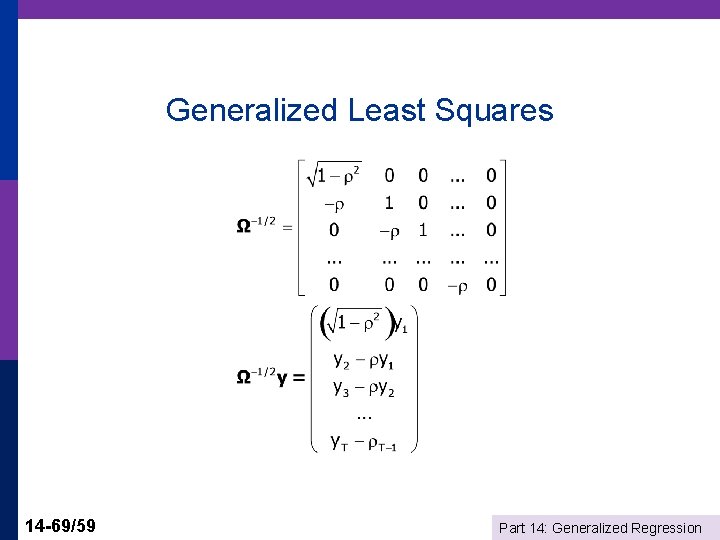
Generalized Least Squares 14 -69/59 Part 14: Generalized Regression

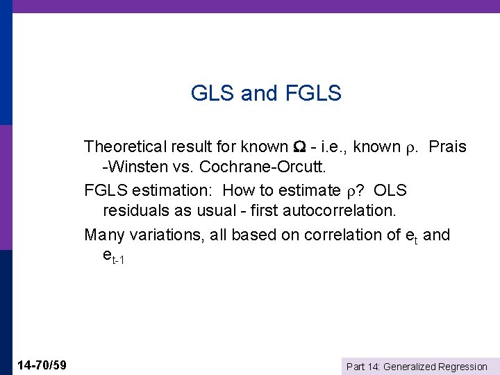
GLS and FGLS Theoretical result for known - i. e. , known . Prais -Winsten vs. Cochrane-Orcutt. FGLS estimation: How to estimate ? OLS residuals as usual - first autocorrelation. Many variations, all based on correlation of et and et-1 14 -70/59 Part 14: Generalized Regression

The Autoregressive Transformation 14 -71/59 Part 14: Generalized Regression

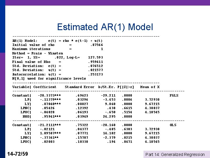
Estimated AR(1) Model -----------------------------------AR(1) Model: e(t) = rho * e(t-1) + u(t) Initial value of rho =. 87566 Maximum iterations = 1 Method = Prais - Winsten Iter= 1, SS=. 022, Log-L= 127. 593 Final value of Rho =. 959411 Std. Deviation: e(t) =. 076512 Std. Deviation: u(t) =. 021577 Autocorrelation: u(t) =. 253173 N[0, 1] used for significance levels ----+------------------------------Variable| Coefficient Standard Error b/St. Er. P[|Z|>z] Mean of X ----+------------------------------------Constant| -20. 3373***. 69623 -29. 211. 0000 FGLS LP| -. 11379***. 03296 -3. 453. 0006 3. 72930 LY|. 87040***. 08827 9. 860. 0000 9. 67215 LPNC|. 05426. 12392. 438. 6615 4. 38037 LPUC| -. 04028. 06193 -. 650. 5154 4. 10545 RHO|. 95941***. 03949 24. 295. 0000 ----+------------------------------------Constant| -21. 2111***. 75322 -28. 160. 0000 OLS LP| -. 02121. 04377 -. 485. 6303 3. 72930 LY| 1. 09587***. 07771 14. 102. 0000 9. 67215 LPNC| -. 37361**. 15707 -2. 379. 0215 4. 38037 LPUC|. 02003. 10330. 194. 8471 4. 10545 14 -72/59 Part 14: Generalized Regression

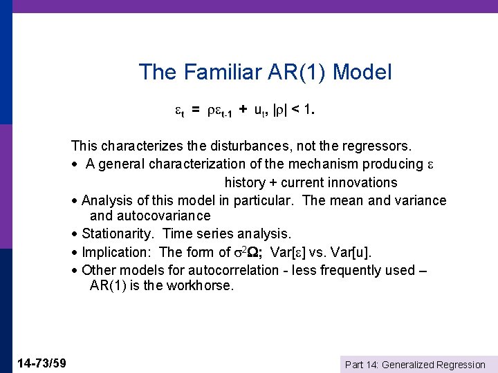
The Familiar AR(1) Model t = t-1 + ut, | | < 1. This characterizes the disturbances, not the regressors. A general characterization of the mechanism producing history + current innovations Analysis of this model in particular. The mean and variance and autocovariance Stationarity. Time series analysis. Implication: The form of 2 ; Var[ ] vs. Var[u]. Other models for autocorrelation - less frequently used – AR(1) is the workhorse. 14 -73/59 Part 14: Generalized Regression

Building the Model p Prior view: A feature of the data n n p “Account for autocorrelation in the data. ” Different models, different estimators Contemporary view: Why is there autocorrelation? n n 14 -74/59 What is missing from the model? Build in appropriate dynamic structures Autocorrelation should be “built out” of the model Use robust procedures (Newey-West) instead of elaborate models specifically for the autocorrelation. Part 14: Generalized Regression

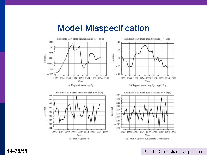
Model Misspecification 14 -75/59 Part 14: Generalized Regression

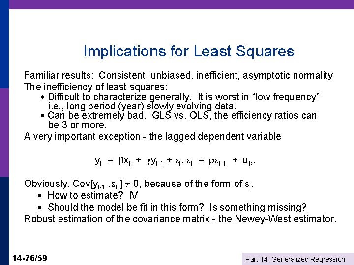
Implications for Least Squares Familiar results: Consistent, unbiased, inefficient, asymptotic normality The inefficiency of least squares: Difficult to characterize generally. It is worst in “low frequency” i. e. , long period (year) slowly evolving data. Can be extremely bad. GLS vs. OLS, the efficiency ratios can be 3 or more. A very important exception - the lagged dependent variable yt = xt + yt-1 + t. t = t-1 + ut, . Obviously, Cov[yt-1 , t ] 0, because of the form of t. How to estimate? IV Should the model be fit in this form? Is something missing? Robust estimation of the covariance matrix - the Newey-West estimator. 14 -76/59 Part 14: Generalized Regression

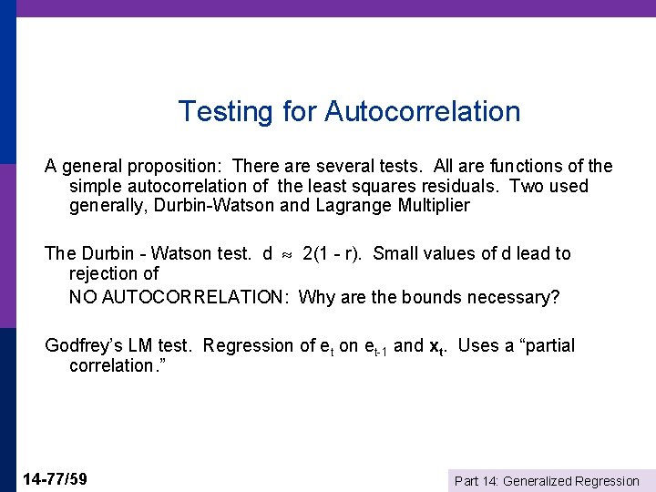
Testing for Autocorrelation A general proposition: There are several tests. All are functions of the simple autocorrelation of the least squares residuals. Two used generally, Durbin-Watson and Lagrange Multiplier The Durbin - Watson test. d 2(1 - r). Small values of d lead to rejection of NO AUTOCORRELATION: Why are the bounds necessary? Godfrey’s LM test. Regression of et on et-1 and xt. Uses a “partial correlation. ” 14 -77/59 Part 14: Generalized Regression

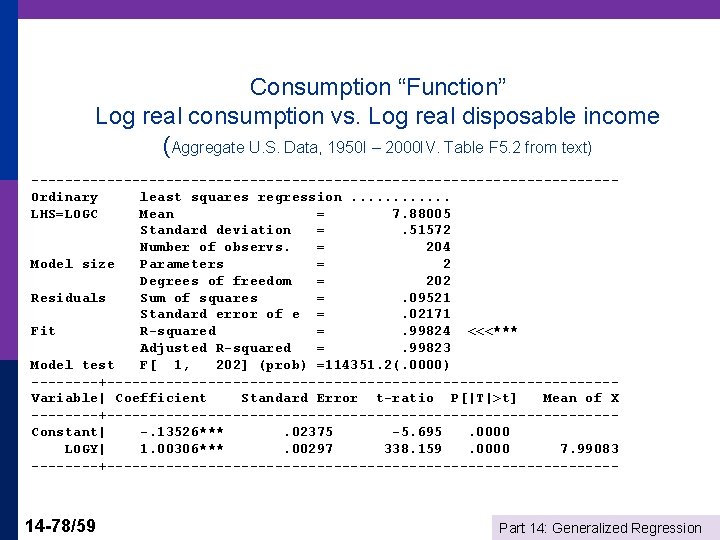
Consumption “Function” Log real consumption vs. Log real disposable income (Aggregate U. S. Data, 1950 I – 2000 IV. Table F 5. 2 from text) -----------------------------------Ordinary least squares regression. . . LHS=LOGC Mean = 7. 88005 Standard deviation =. 51572 Number of observs. = 204 Model size Parameters = 2 Degrees of freedom = 202 Residuals Sum of squares =. 09521 Standard error of e =. 02171 Fit R-squared =. 99824 <<<*** Adjusted R-squared =. 99823 Model test F[ 1, 202] (prob) =114351. 2(. 0000) ----+------------------------------Variable| Coefficient Standard Error t-ratio P[|T|>t] Mean of X ----+------------------------------Constant| -. 13526***. 02375 -5. 695. 0000 LOGY| 1. 00306***. 00297 338. 159. 0000 7. 99083 ----+------------------------------- 14 -78/59 Part 14: Generalized Regression

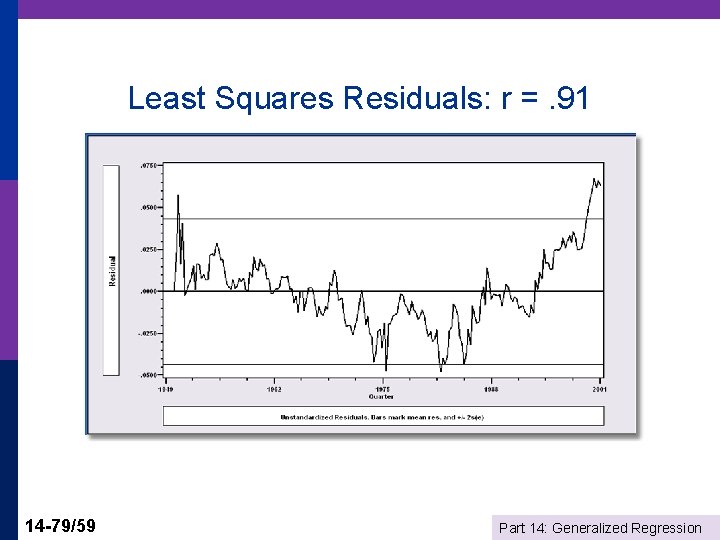
Least Squares Residuals: r =. 91 14 -79/59 Part 14: Generalized Regression

Conventional vs. Newey-West +--------------+--------+---------+-----+ |Variable | Coefficient | Standard Error |t-ratio |P[|T|>t] | Mean of X| +--------------+--------+---------+-----+ Constant -. 13525584. 02375149 -5. 695. 0000 LOGY 1. 00306313. 00296625 338. 159. 0000 7. 99083133 +--------------+--------+---------+-----+ |Newey-West Robust Covariance Matrix |Variable | Coefficient | Standard Error |t-ratio |P[|T|>t] | Mean of X| +--------------+--------+---------+-----+ Constant -. 13525584. 07257279 -1. 864. 0638 LOGY 1. 00306313. 00938791 106. 846. 0000 7. 99083133 14 -80/59 Part 14: Generalized Regression

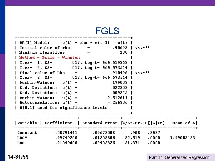
FGLS +-----------------------+ | AR(1) Model: e(t) = rho * e(t-1) + u(t) | | Initial value of rho =. 90693 | <<<*** | Maximum iterations = 100 | | Method = Prais - Winsten | | Iter= 1, SS=. 017, Log-L= 666. 519353 | | Iter= 2, SS=. 017, Log-L= 666. 573544 | | Final value of Rho =. 910496 | <<<*** | Iter= 2, SS=. 017, Log-L= 666. 573544 | | Durbin-Watson: e(t) =. 179008 | | Std. Deviation: e(t) =. 022308 | | Std. Deviation: u(t) =. 009225 | | Durbin-Watson: u(t) = 2. 512611 | | Autocorrelation: u(t) = -. 256306 | | N[0, 1] used for significance levels | +-----------------------+ +--------------+--------+---------+-----+ |Variable | Coefficient | Standard Error |b/St. Er. |P[|Z|>z] | Mean of X| +--------------+--------+---------+-----+ Constant -. 08791441. 09678008 -. 908. 3637 LOGY. 99749200. 01208806 82. 519. 0000 7. 99083133 RHO. 91049600. 02902326 31. 371. 0000 14 -81/59 Part 14: Generalized Regression

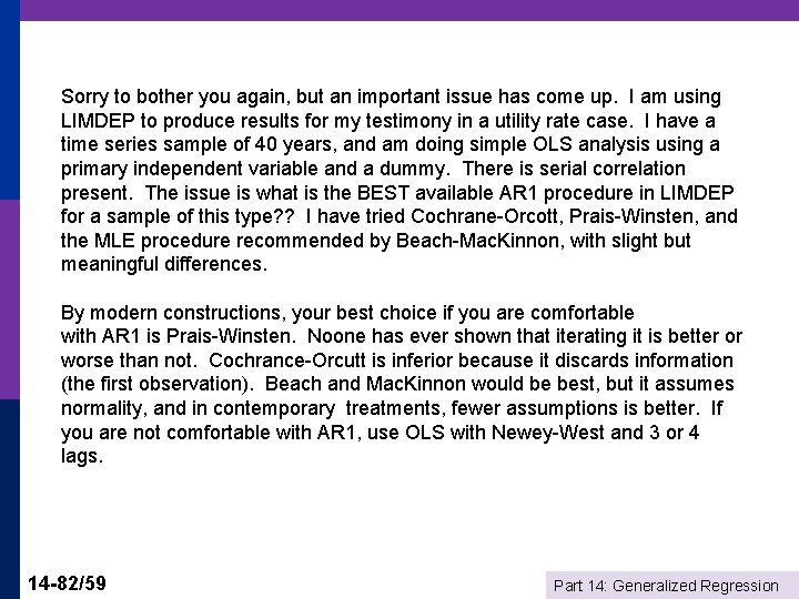
Sorry to bother you again, but an important issue has come up. I am using LIMDEP to produce results for my testimony in a utility rate case. I have a time series sample of 40 years, and am doing simple OLS analysis using a primary independent variable and a dummy. There is serial correlation present. The issue is what is the BEST available AR 1 procedure in LIMDEP for a sample of this type? ? I have tried Cochrane-Orcott, Prais-Winsten, and the MLE procedure recommended by Beach-Mac. Kinnon, with slight but meaningful differences. By modern constructions, your best choice if you are comfortable with AR 1 is Prais-Winsten. Noone has ever shown that iterating it is better or worse than not. Cochrance-Orcutt is inferior because it discards information (the first observation). Beach and Mac. Kinnon would be best, but it assumes normality, and in contemporary treatments, fewer assumptions is better. If you are not comfortable with AR 1, use OLS with Newey-West and 3 or 4 lags. 14 -82/59 Part 14: Generalized Regression

Feasible GLS 14 -83/59 Part 14: Generalized Regression