Econometrics I Professor William Greene Stern School of

Econometrics I Professor William Greene Stern School of Business Department of Economics 24 -/35 Part 24: Bayesian Estimation

Econometrics I Part 24 – Bayesian Estimation 24 -/35 Part 24: Bayesian Estimation

Bayesian Estimators “Random Parameters” vs. Randomly Distributed Parameters p Models of Individual Heterogeneity p n n 24 -3/35 Random Effects: Consumer Brand Choice Fixed Effects: Hospital Costs Part 24: Bayesian Estimation

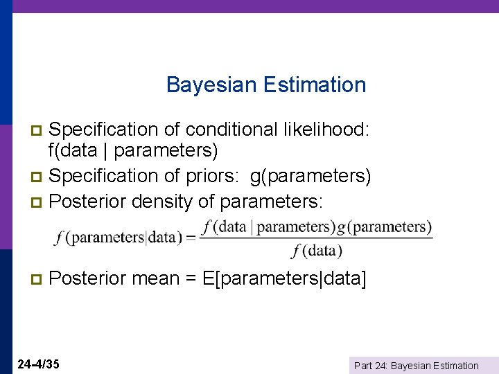
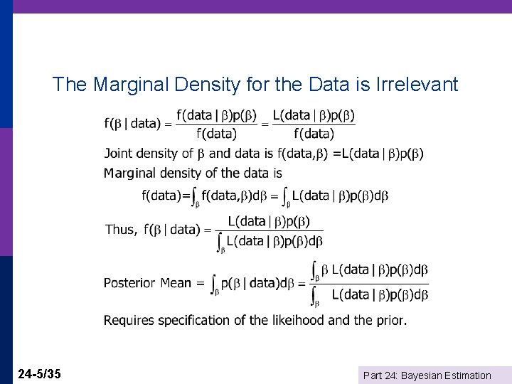
Bayesian Estimation Specification of conditional likelihood: f(data | parameters) p Specification of priors: g(parameters) p Posterior density of parameters: p p Posterior mean = E[parameters|data] 24 -4/35 Part 24: Bayesian Estimation

The Marginal Density for the Data is Irrelevant 24 -5/35 Part 24: Bayesian Estimation

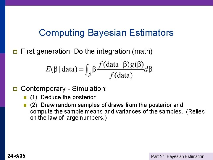
Computing Bayesian Estimators p First generation: Do the integration (math) p Contemporary - Simulation: n n 24 -6/35 (1) Deduce the posterior (2) Draw random samples of draws from the posterior and compute the sample means and variances of the samples. (Relies on the law of large numbers. ) Part 24: Bayesian Estimation

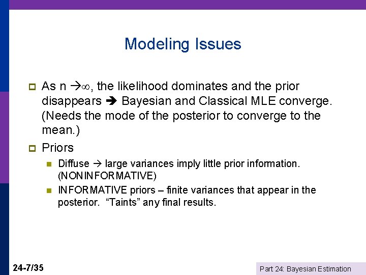
Modeling Issues p p As n , the likelihood dominates and the prior disappears Bayesian and Classical MLE converge. (Needs the mode of the posterior to converge to the mean. ) Priors n n 24 -7/35 Diffuse large variances imply little prior information. (NONINFORMATIVE) INFORMATIVE priors – finite variances that appear in the posterior. “Taints” any final results. Part 24: Bayesian Estimation

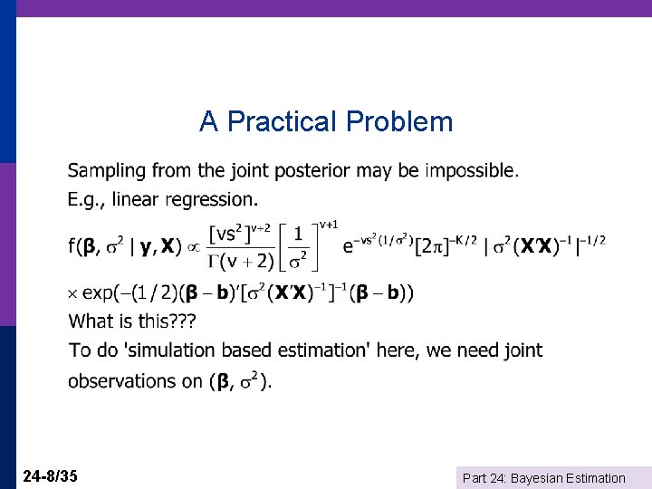
A Practical Problem 24 -8/35 Part 24: Bayesian Estimation

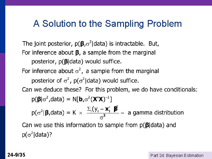
A Solution to the Sampling Problem 24 -9/35 Part 24: Bayesian Estimation

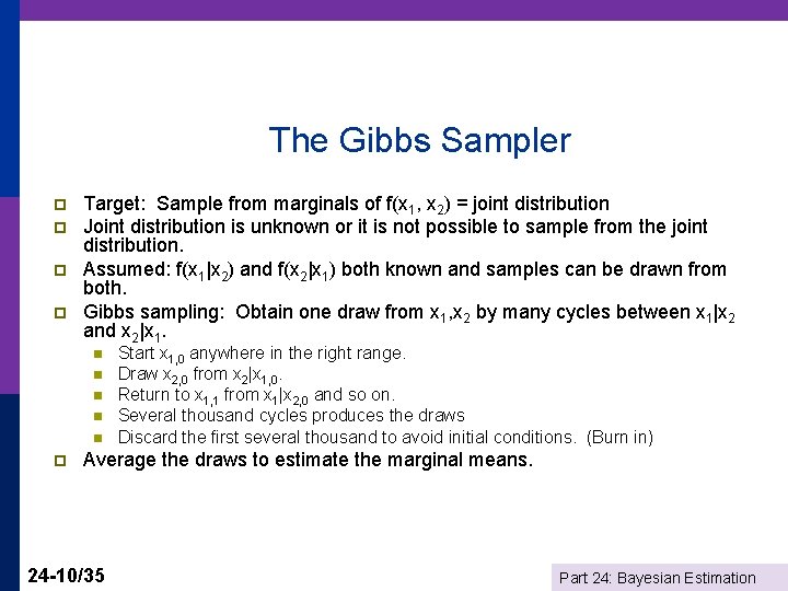
The Gibbs Sampler p p Target: Sample from marginals of f(x 1, x 2) = joint distribution Joint distribution is unknown or it is not possible to sample from the joint distribution. Assumed: f(x 1|x 2) and f(x 2|x 1) both known and samples can be drawn from both. Gibbs sampling: Obtain one draw from x 1, x 2 by many cycles between x 1|x 2 and x 2|x 1. n n n p Start x 1, 0 anywhere in the right range. Draw x 2, 0 from x 2|x 1, 0. Return to x 1, 1 from x 1|x 2, 0 and so on. Several thousand cycles produces the draws Discard the first several thousand to avoid initial conditions. (Burn in) Average the draws to estimate the marginal means. 24 -10/35 Part 24: Bayesian Estimation

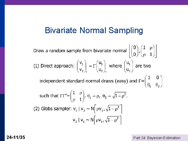
Bivariate Normal Sampling 24 -11/35 Part 24: Bayesian Estimation

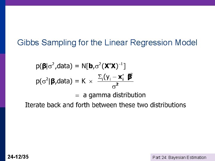
Gibbs Sampling for the Linear Regression Model 24 -12/35 Part 24: Bayesian Estimation

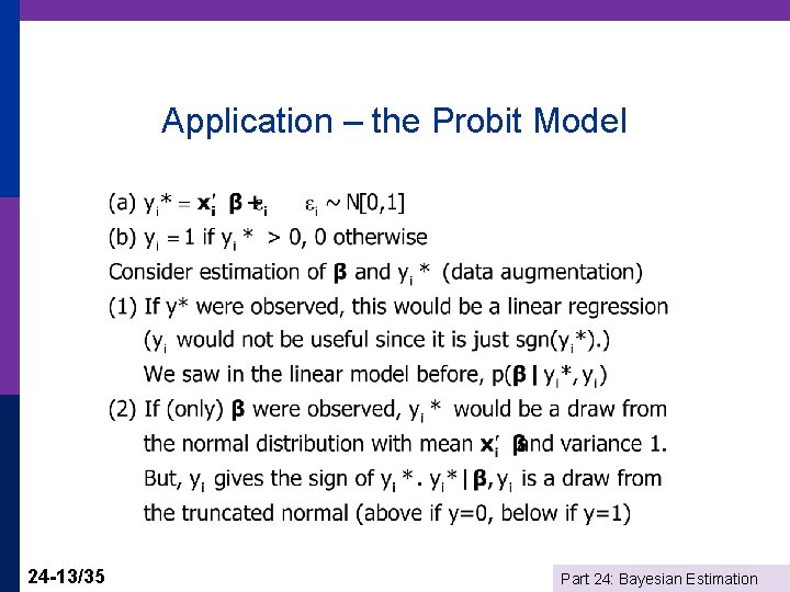
Application – the Probit Model 24 -13/35 Part 24: Bayesian Estimation

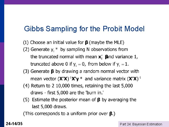
Gibbs Sampling for the Probit Model 24 -14/35 Part 24: Bayesian Estimation

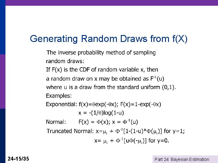
Generating Random Draws from f(X) 24 -15/35 Part 24: Bayesian Estimation

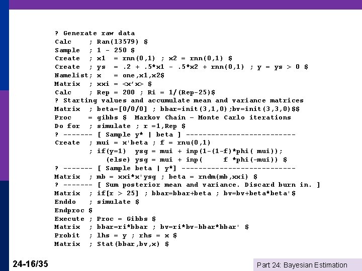
? Generate raw data Calc ; Ran(13579) $ Sample ; 1 - 250 $ Create ; x 1 = rnn(0, 1) ; x 2 = rnn(0, 1) $ Create ; ys =. 2 +. 5*x 1 -. 5*x 2 + rnn(0, 1) ; y = ys > 0 $ Namelist; x = one, x 1, x 2$ Matrix ; xxi = <x’x> $ Calc ; Rep = 200 ; Ri = 1/(Rep-25)$ ? Starting values and accumulate mean and variance matrices Matrix ; beta=[0/0/0] ; bbar=init(3, 1, 0); bv=init(3, 3, 0)$$ Proc = gibbs $ Markov Chain – Monte Carlo iterations Do for ; simulate ; r =1, Rep $ ? ------- [ Sample y* | beta ] -------------Create ; mui = x'beta ; f = rnu(0, 1) ; if(y=1) ysg = mui + inp(1 -(1 -f)*phi( mui)); (else) ysg = mui + inp( f *phi(-mui)) $ ? ------- [ Sample beta | y*] -------------Matrix ; mb = xxi*x'ysg ; beta = rndm(mb, xxi) $ ? ------- [ Sum posterior mean and variance. Discard burn in. ] Matrix ; if[r > 25] ; bbar=bbar+beta ; bv=bv+beta*beta'$ Enddo ; simulate $ Endproc $ Execute ; Proc = Gibbs $ Matrix ; bbar=ri*bbar ; bv=ri*bv-bbar*bbar' $ Probit ; lhs = y ; rhs = x $ Matrix ; Stat(bbar, bv, x) $ 24 -16/35 Part 24: Bayesian Estimation

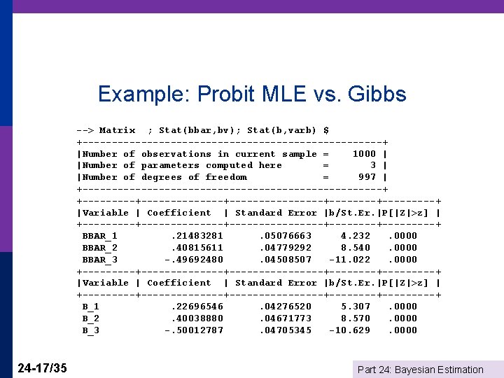
Example: Probit MLE vs. Gibbs --> Matrix ; Stat(bbar, bv); Stat(b, varb) $ +--------------------------+ |Number of observations in current sample = 1000 | |Number of parameters computed here = 3 | |Number of degrees of freedom = 997 | +--------------------------+ +--------------+--------+---------+ |Variable | Coefficient | Standard Error |b/St. Er. |P[|Z|>z] | +--------------+--------+---------+ BBAR_1. 21483281. 05076663 4. 232. 0000 BBAR_2. 40815611. 04779292 8. 540. 0000 BBAR_3 -. 49692480. 04508507 -11. 022. 0000 +--------------+--------+---------+ |Variable | Coefficient | Standard Error |b/St. Er. |P[|Z|>z] | +--------------+--------+---------+ B_1. 22696546. 04276520 5. 307. 0000 B_2. 40038880. 04671773 8. 570. 0000 B_3 -. 50012787. 04705345 -10. 629. 0000 24 -17/35 Part 24: Bayesian Estimation

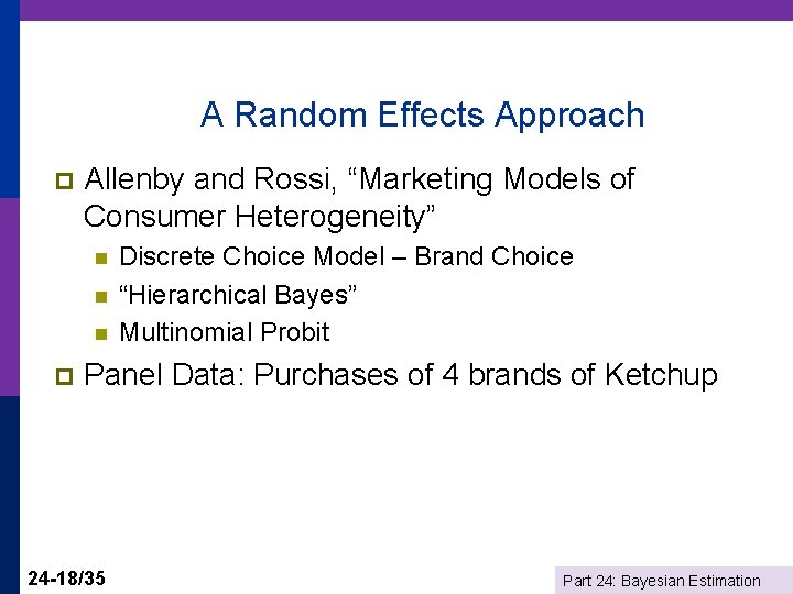
A Random Effects Approach p Allenby and Rossi, “Marketing Models of Consumer Heterogeneity” n n n p Discrete Choice Model – Brand Choice “Hierarchical Bayes” Multinomial Probit Panel Data: Purchases of 4 brands of Ketchup 24 -18/35 Part 24: Bayesian Estimation

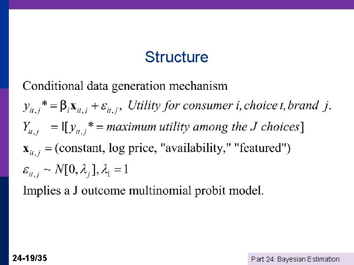
Structure 24 -19/35 Part 24: Bayesian Estimation

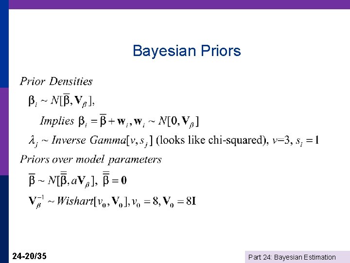
Bayesian Priors 24 -20/35 Part 24: Bayesian Estimation

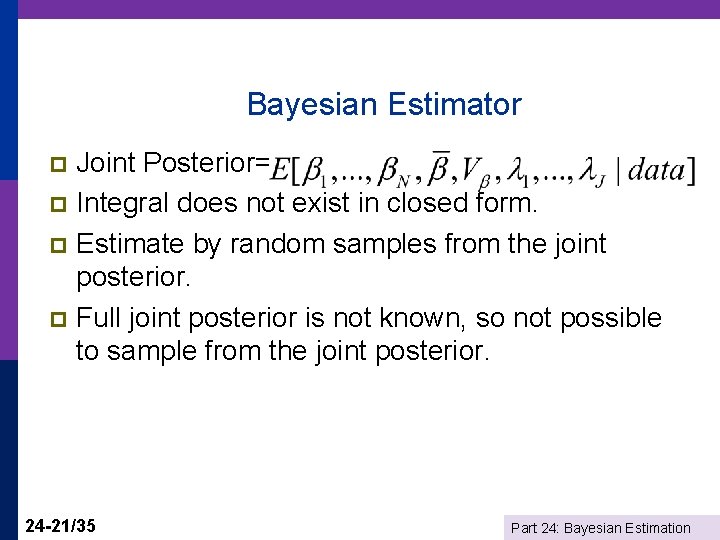
Bayesian Estimator Joint Posterior= p Integral does not exist in closed form. p Estimate by random samples from the joint posterior. p Full joint posterior is not known, so not possible to sample from the joint posterior. p 24 -21/35 Part 24: Bayesian Estimation

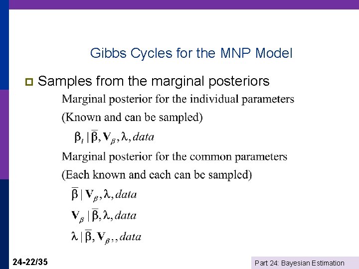
Gibbs Cycles for the MNP Model p Samples from the marginal posteriors 24 -22/35 Part 24: Bayesian Estimation

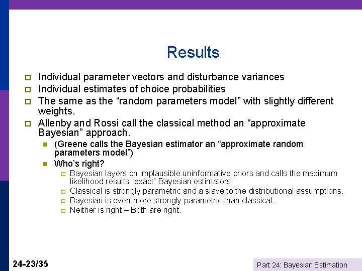
Results p p Individual parameter vectors and disturbance variances Individual estimates of choice probabilities The same as the “random parameters model” with slightly different weights. Allenby and Rossi call the classical method an “approximate Bayesian” approach. n n (Greene calls the Bayesian estimator an “approximate random parameters model”) Who’s right? p p 24 -23/35 Bayesian layers on implausible uninformative priors and calls the maximum likelihood results “exact” Bayesian estimators Classical is strongly parametric and a slave to the distributional assumptions. Bayesian is even more strongly parametric than classical. Neither is right – Both are right. Part 24: Bayesian Estimation

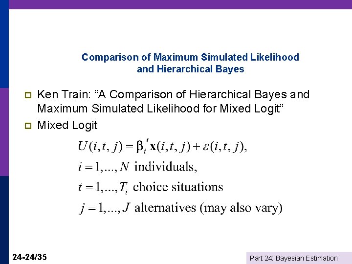
Comparison of Maximum Simulated Likelihood and Hierarchical Bayes p p Ken Train: “A Comparison of Hierarchical Bayes and Maximum Simulated Likelihood for Mixed Logit” Mixed Logit 24 -24/35 Part 24: Bayesian Estimation

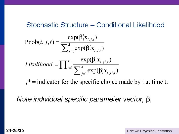
Stochastic Structure – Conditional Likelihood Note individual specific parameter vector, i 24 -25/35 Part 24: Bayesian Estimation

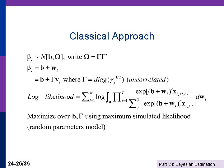
Classical Approach 24 -26/35 Part 24: Bayesian Estimation

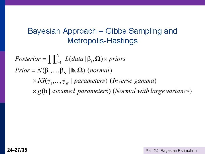
Bayesian Approach – Gibbs Sampling and Metropolis-Hastings 24 -27/35 Part 24: Bayesian Estimation

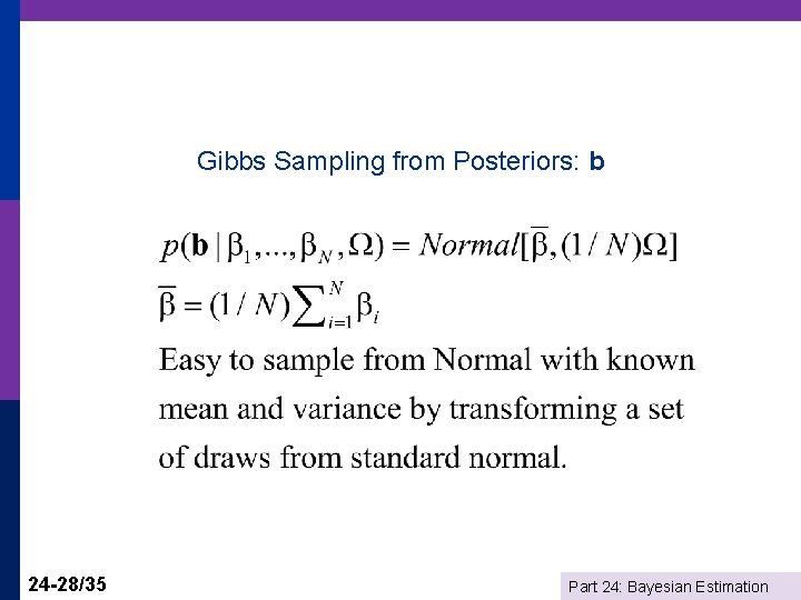
Gibbs Sampling from Posteriors: b 24 -28/35 Part 24: Bayesian Estimation

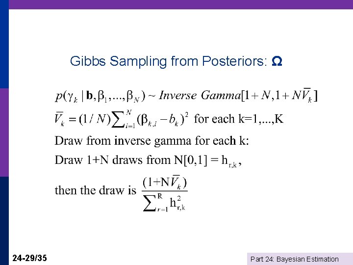
Gibbs Sampling from Posteriors: Ω 24 -29/35 Part 24: Bayesian Estimation

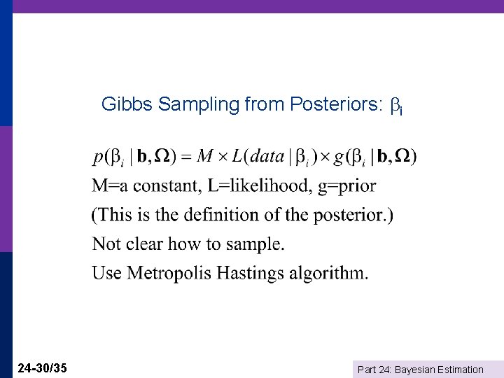
Gibbs Sampling from Posteriors: i 24 -30/35 Part 24: Bayesian Estimation

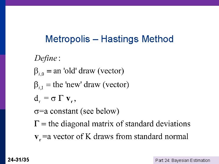
Metropolis – Hastings Method 24 -31/35 Part 24: Bayesian Estimation

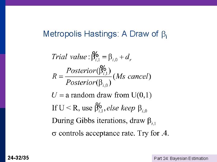
Metropolis Hastings: A Draw of i 24 -32/35 Part 24: Bayesian Estimation

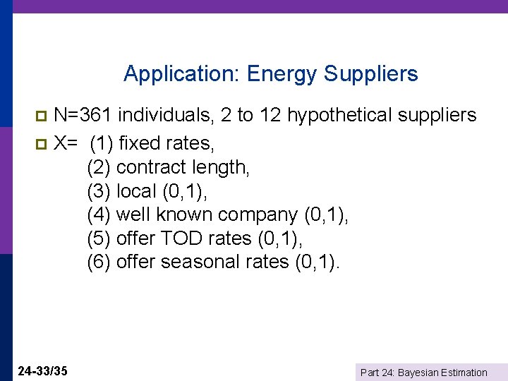
Application: Energy Suppliers N=361 individuals, 2 to 12 hypothetical suppliers p X= (1) fixed rates, (2) contract length, (3) local (0, 1), (4) well known company (0, 1), (5) offer TOD rates (0, 1), (6) offer seasonal rates (0, 1). p 24 -33/35 Part 24: Bayesian Estimation

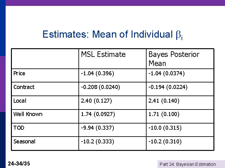
Estimates: Mean of Individual i MSL Estimate Bayes Posterior Mean Price -1. 04 (0. 396) -1. 04 (0. 0374) Contract -0. 208 (0. 0240) -0. 194 (0. 0224) Local 2. 40 (0. 127) 2. 41 (0. 140) Well Known 1. 74 (0. 0927) 1. 71 (0. 100) TOD -9. 94 (0. 337) -10. 0 (0. 315) Seasonal -10. 2 (0. 333) -10. 2 (0. 310) 24 -34/35 Part 24: Bayesian Estimation

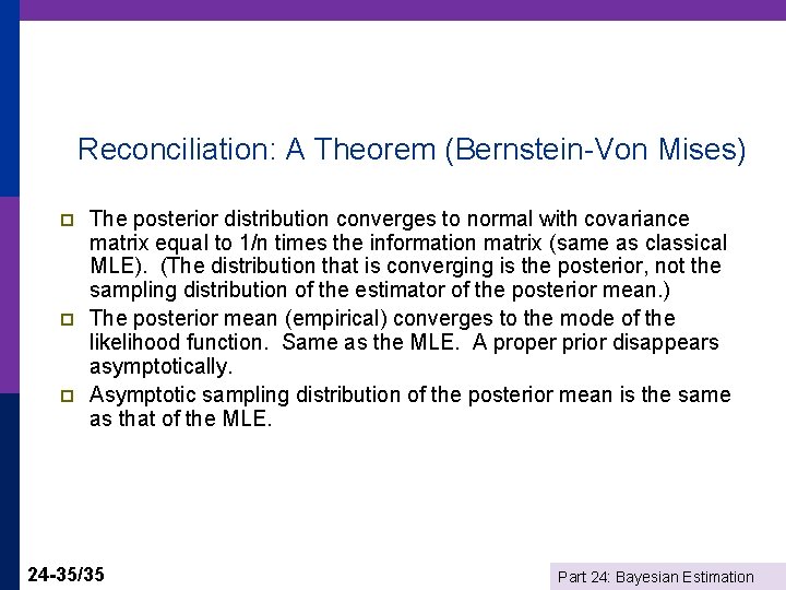
Reconciliation: A Theorem (Bernstein-Von Mises) p p p The posterior distribution converges to normal with covariance matrix equal to 1/n times the information matrix (same as classical MLE). (The distribution that is converging is the posterior, not the sampling distribution of the estimator of the posterior mean. ) The posterior mean (empirical) converges to the mode of the likelihood function. Same as the MLE. A proper prior disappears asymptotically. Asymptotic sampling distribution of the posterior mean is the same as that of the MLE. 24 -35/35 Part 24: Bayesian Estimation