Weather Derivatives Dr Harvey Stern Climate Manager Victoria

Weather Derivatives Dr Harvey Stern, Climate Manager, Victoria

Introduction Evidence of the challenge faced by the meteorological community to become skilled in applying risk management products from financial markets is growing. An empirical approach to the pricing of weather derivatives is presented. The approach is illustrated with several examples.

Background It is the energy and power industry that has, so far, taken best advantage of the opportunities presented by weather derivatives. Indeed, the first weather derivative contract was a temperature-related power swap transacted in August 1996.

Weather Derivatives Defined Clewlow et al. . . (2000) describe weather derivatives as being similar "to conventional financial derivatives, the basic difference coming from the underlying variables that determine the pay-offs", such as temperature, precipitation, wind, heating degree days, and cooling degree days.

Defining Cooling Degree Days Number of cooling degree days during a season is the accumulated number of degrees the daily mean temperature is above a base figure, usually 18 deg C. Number of cooling degree days might be regarded as a measure of the requirement for cooling.

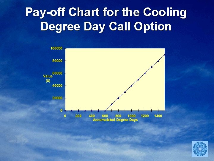
Defining a Cooling Degree Day Call Option • Strike: 600 cooling degree days. • Notional: $100 per cooling degree day (above 600). If, at the expiry of this contract, the accumulated number of cooling degree days is greater than 600, then the seller of the option pays the buyer $100 for each cooling degree day above 600.

Pay-off Chart for the Cooling Degree Day Call Option

Pricing Approaches • Historical simulation. • Direct modeling of the underlying variable’s distribution. • Indirect modeling of the underlying variable’s distribution (this involves simulating a sequence of data).

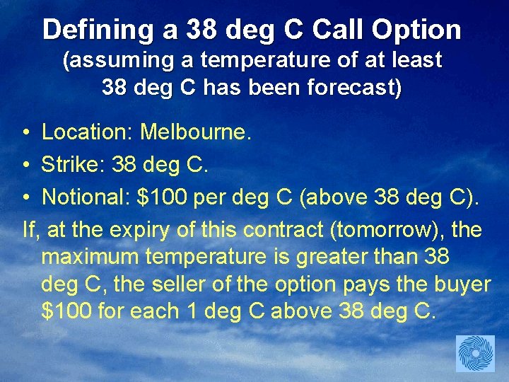
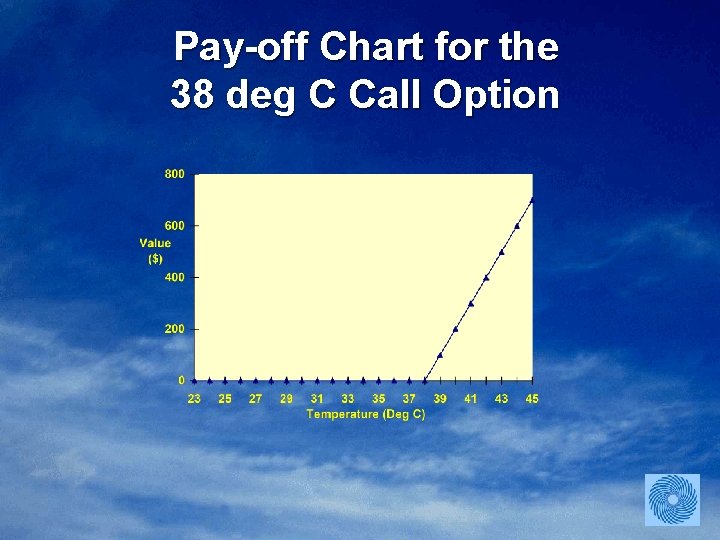
Defining a 38 deg C Call Option (assuming a temperature of at least 38 deg C has been forecast) • Location: Melbourne. • Strike: 38 deg C. • Notional: $100 per deg C (above 38 deg C). If, at the expiry of this contract (tomorrow), the maximum temperature is greater than 38 deg C, the seller of the option pays the buyer $100 for each 1 deg C above 38 deg C.

Pay-off Chart for the 38 deg C Call Option

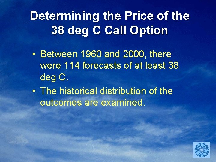
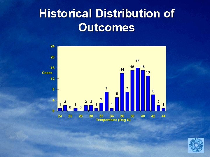
Determining the Price of the 38 deg C Call Option • Between 1960 and 2000, there were 114 forecasts of at least 38 deg C. • The historical distribution of the outcomes are examined.

Historical Distribution of Outcomes

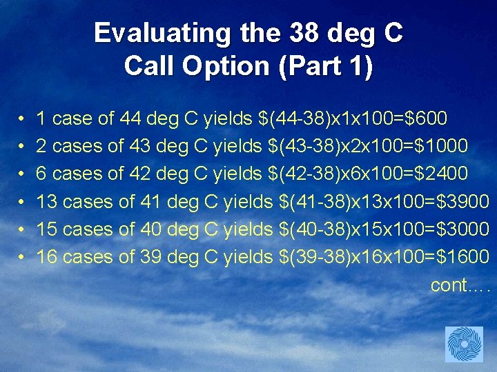
Evaluating the 38 deg C Call Option (Part 1) • • • 1 case of 44 deg C yields $(44 -38)x 1 x 100=$600 2 cases of 43 deg C yields $(43 -38)x 2 x 100=$1000 6 cases of 42 deg C yields $(42 -38)x 6 x 100=$2400 13 cases of 41 deg C yields $(41 -38)x 13 x 100=$3900 15 cases of 40 deg C yields $(40 -38)x 15 x 100=$3000 16 cases of 39 deg C yields $(39 -38)x 16 x 100=$1600 cont….

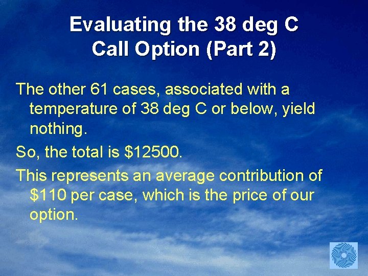
Evaluating the 38 deg C Call Option (Part 2) The other 61 cases, associated with a temperature of 38 deg C or below, yield nothing. So, the total is $12500. This represents an average contribution of $110 per case, which is the price of our option.

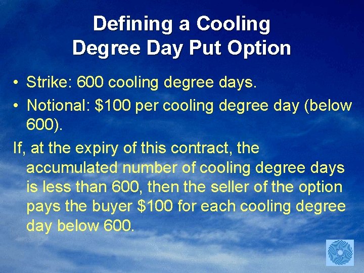
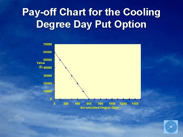
Defining a Cooling Degree Day Put Option • Strike: 600 cooling degree days. • Notional: $100 per cooling degree day (below 600). If, at the expiry of this contract, the accumulated number of cooling degree days is less than 600, then the seller of the option pays the buyer $100 for each cooling degree day below 600.

Pay-off Chart for the Cooling Degree Day Put Option

A Forecast Error Put Option (defining error as predicted minus observed) • Strike: 0 deg C. • Notional: $100 per degree of forecast error below 0 deg C If the forecast underestimates the actual temperature, then the seller of the option pays the buyer $100 for each 1 deg C of underestimation.

Evaluating the Forecast Error Put Option • Historical simulation yields a suggested price of $67 for our put option. Two questions: • Does today’s error influence the price? • Does tomorrow’s expected weather pattern influence the price?

Answering the First Question Today’s error does influence the price: If today’s forecast is an underestimate, then tomorrow’s is also likely to be an underestimate, leading to a suggested option price of $75. If today’s forecast is an overestimate, then tomorrow’s is also likely to be, leading to a suggested option price of $41.

Answering the Second Question Tomorrow’s weather pattern does influence the price, for example: If tomorrow’s weather pattern is moderate anticyclonic NNE, tomorrow’s forecast is likely to be an underestimate, leading to a price of $77. However, if tomorrow’s weather pattern is strong anticyclonic NNE, tomorrow’s forecast is likely to be an overestimate, leading to a price of $47.

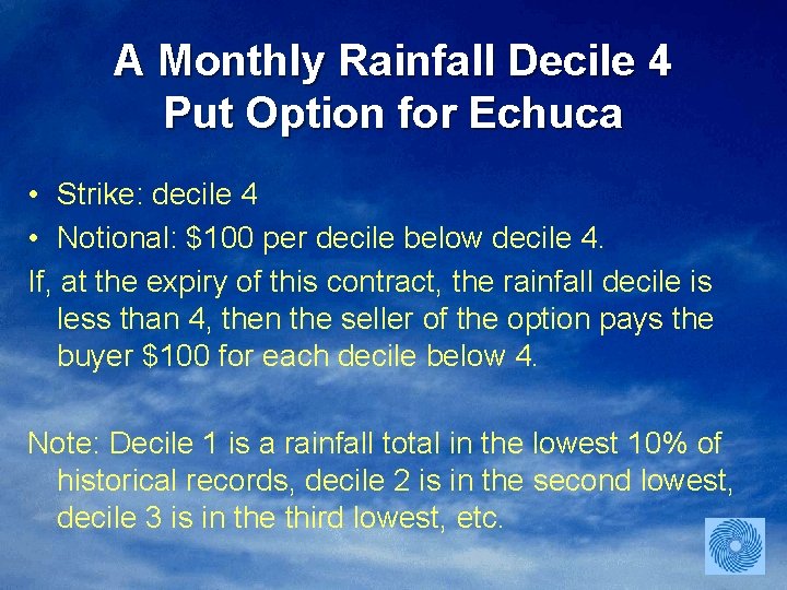
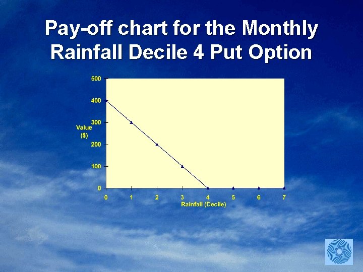
A Monthly Rainfall Decile 4 Put Option for Echuca • Strike: decile 4 • Notional: $100 per decile below decile 4. If, at the expiry of this contract, the rainfall decile is less than 4, then the seller of the option pays the buyer $100 for each decile below 4. Note: Decile 1 is a rainfall total in the lowest 10% of historical records, decile 2 is in the second lowest, decile 3 is in the third lowest, etc.

Pay-off chart for the Monthly Rainfall Decile 4 Put Option

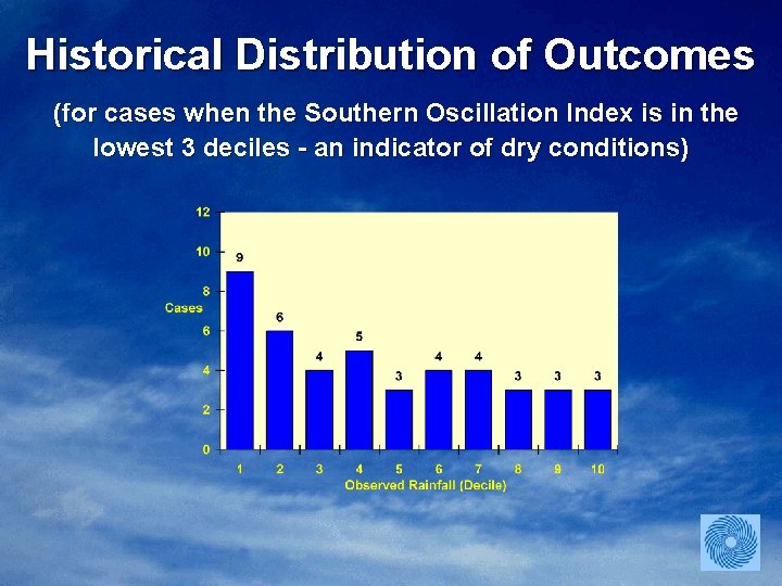
Historical Distribution of Outcomes (for cases when the Southern Oscillation Index is in the lowest 3 deciles - an indicator of dry conditions)

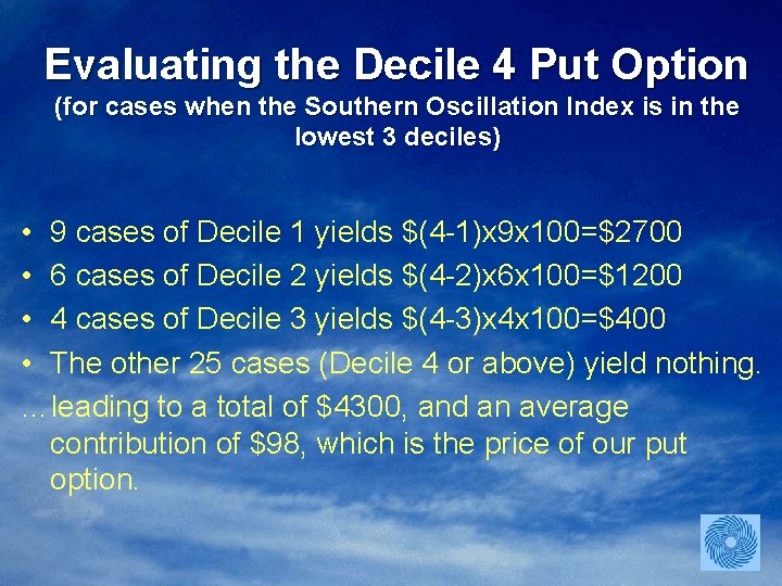
Evaluating the Decile 4 Put Option (for cases when the Southern Oscillation Index is in the lowest 3 deciles) • 9 cases of Decile 1 yields $(4 -1)x 9 x 100=$2700 • 6 cases of Decile 2 yields $(4 -2)x 6 x 100=$1200 • 4 cases of Decile 3 yields $(4 -3)x 4 x 100=$400 • The other 25 cases (Decile 4 or above) yield nothing. …leading to a total of $4300, and an average contribution of $98, which is the price of our put option.

Evaluating Other Derivatives An experiment is conducted to illustrate the importance of mean reversion and jumps in the evaluation of other financial derivatives. Mean reversion and jumps are features of the Monte Carlo approach to modeling weather derivatives.

The Experiment It is assumed that stocks are purchased following a break in an extended sequence of consecutive price falls. It is assumed that stocks are short-sold following a break in an extended sequence of consecutive price rises. Net returns are determined.

Mean Reversion Mean reversion is demonstrated by: The average return being +4. 51% with a standard deviation of 12. 15% yielding the result. The average is different from zero at the 0. 1% level of significance, the +ve return reflecting the operation of mean reversion.

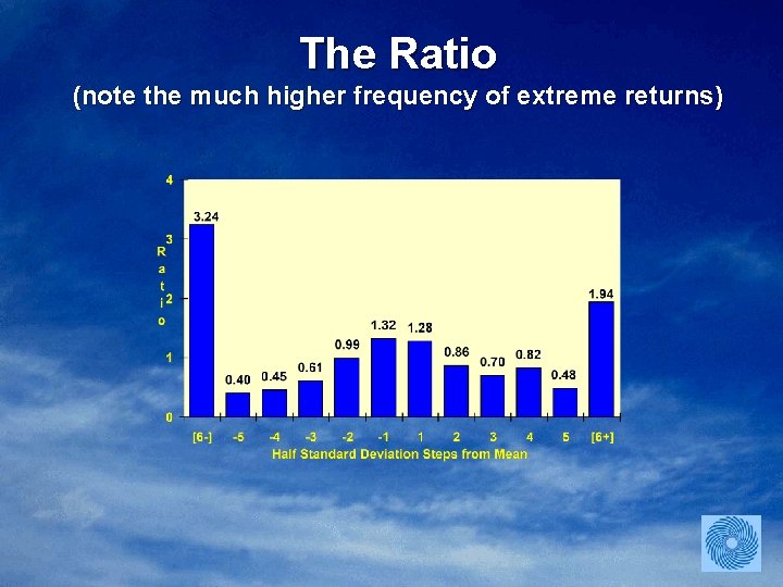
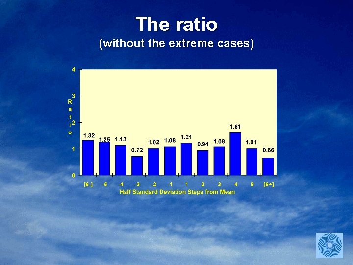
Jumps The operation of jumps is illustrated in the next slide, which presents the ratio: (frequency of returns from experiment) (frequency of returns if distribution normal) that ratio being presented in half standard deviation steps from the mean.

The Ratio (note the much higher frequency of extreme returns)

The ratio (without the extreme cases)

Concluding Remarks • An empirical approach to the pricing of weather derivatives has been presented. • The approach utilises a range of data types to price weather derivatives, including forecast accuracy data. • It has been shown that mean reversion and jumps, features of the Monte Carlo approach to the modeling of weather derivatives, should also be included in the modeling of other derivatives.

To view the presentation again … Go to: http: //www. weather-climate. com/derivatives. ppt