Econometrics I Professor William Greene Stern School of

Econometrics I Professor William Greene Stern School of Business Department of Economics 3 -/29 Part 3: Least Squares Algebra

Econometrics I Part 3 – Least Squares Algebra 3 -/29 Part 3: Least Squares Algebra

Vocabulary p p p 3 -3/29 Some terms to be used in the discussion. n Population characteristics and entities vs. sample quantities and analogs n Residuals and disturbances n Population regression line and sample regression Objective: Learn about the conditional mean function. ‘Estimate’ and 2 First step: Mechanics of fitting a line (hyperplane) to a set of data Part 3: Least Squares Algebra

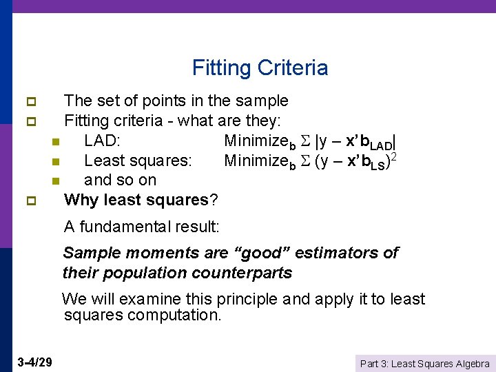
Fitting Criteria p p p The set of points in the sample Fitting criteria - what are they: n LAD: Minimizeb |y – x’b. LAD| n Least squares: Minimizeb (y – x’b. LS)2 n and so on Why least squares? A fundamental result: Sample moments are “good” estimators of their population counterparts We will examine this principle and apply it to least squares computation. 3 -4/29 Part 3: Least Squares Algebra

An Analogy Principle for Estimating In the population E[y | X ] = X so E[y - X |X] = 0 Continuing (assumed) E[xi i] = 0 for every i Summing, Σi E[xi i] = Σi 0 = 0 Exchange Σi and E[] E[Σi xi i] = E[ X ] = 0 E[X (y - X ) ] = 0 So, if X is the conditional mean, then E[X’ ] = 0. We choose b, the estimator of , to mimic this population result: i. e. , mimic the population mean with the sample mean Find b such that As we will see, the solution is the least squares coefficient vector. 3 -5/29 Part 3: Least Squares Algebra

Population Moments We assumed that E[ i|xi] = 0. (Slide 2: 40) It follows that Cov[xi, i] = 0. Proof: Cov(xi, i) = Cov(xi, E[ i |xi]) = Cov(xi, 0) = 0. (Theorem B. 2). If E[yi|xi] = xi’ , then = (Var[xi])-1 Cov[xi, yi]. Proof: Cov[xi, yi] = Cov[xi, E[yi|xi]]=Cov[xi, xi’ ] This will provide a population analog to the statistics we compute with the data. 3 -6/29 Part 3: Least Squares Algebra

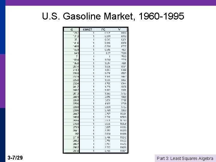
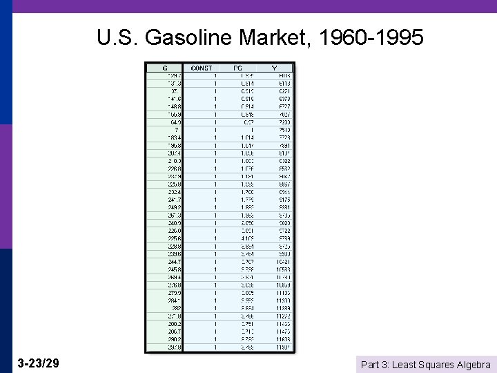
U. S. Gasoline Market, 1960 -1995 3 -7/29 Part 3: Least Squares Algebra

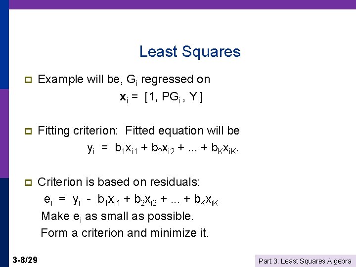
Least Squares p Example will be, Gi regressed on xi = [1, PGi , Yi] p Fitting criterion: Fitted equation will be yi = b 1 xi 1 + b 2 xi 2 +. . . + b. Kxi. K. p Criterion is based on residuals: ei = yi - b 1 xi 1 + b 2 xi 2 +. . . + b. Kxi. K Make ei as small as possible. Form a criterion and minimize it. 3 -8/29 Part 3: Least Squares Algebra

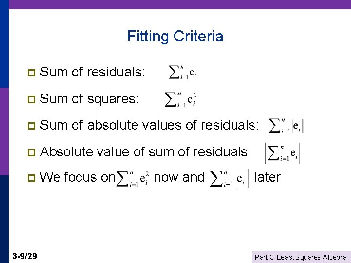
Fitting Criteria p Sum of residuals: p Sum of squares: p Sum of absolute values of residuals: p Absolute value of sum of residuals p We focus on 3 -9/29 now and later Part 3: Least Squares Algebra

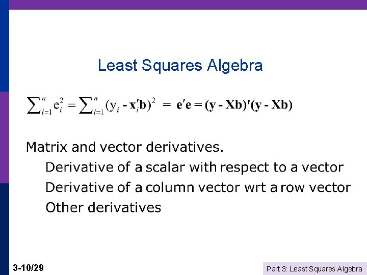
Least Squares Algebra 3 -10/29 Part 3: Least Squares Algebra

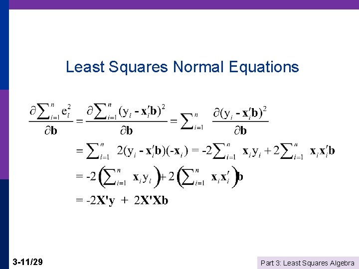
Least Squares Normal Equations 3 -11/29 Part 3: Least Squares Algebra

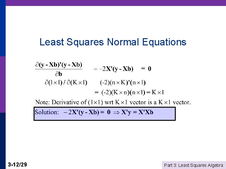
Least Squares Normal Equations 3 -12/29 Part 3: Least Squares Algebra

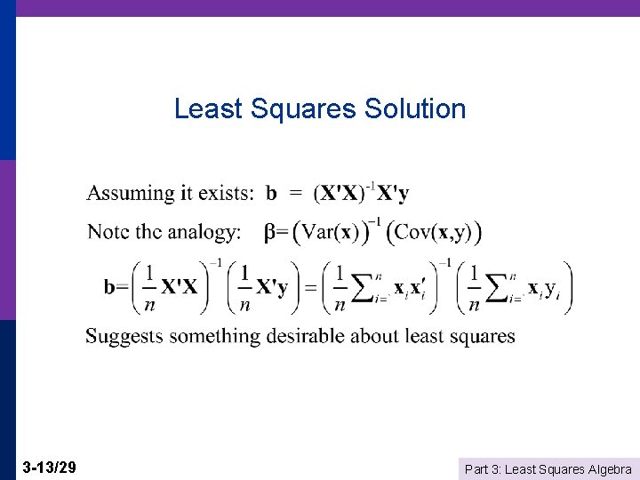
Least Squares Solution 3 -13/29 Part 3: Least Squares Algebra

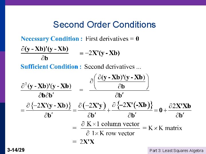
Second Order Conditions 3 -14/29 Part 3: Least Squares Algebra

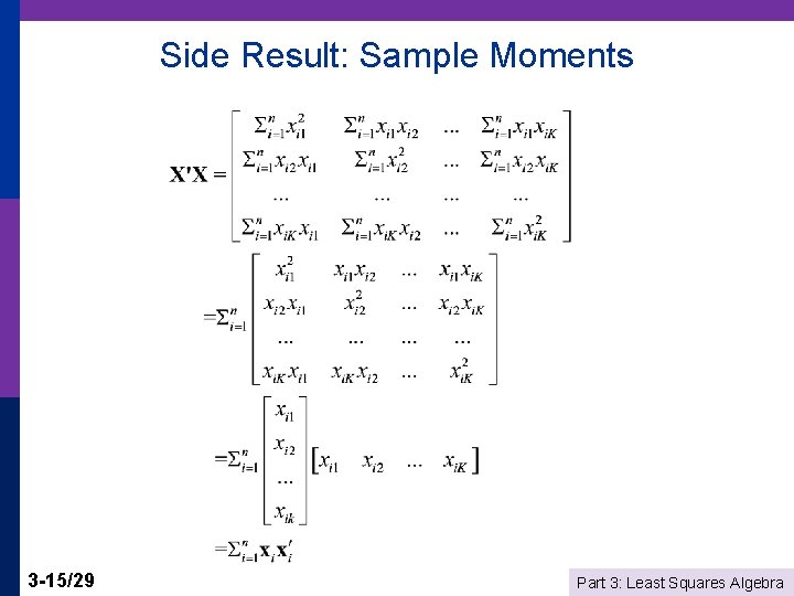
Side Result: Sample Moments 3 -15/29 Part 3: Least Squares Algebra

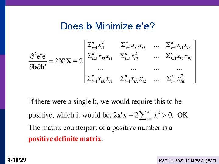
Does b Minimize e’e? 3 -16/29 Part 3: Least Squares Algebra

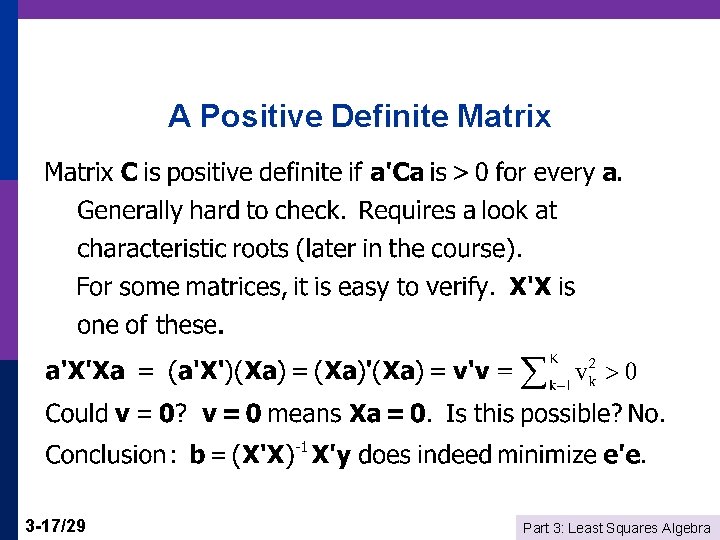
A Positive Definite Matrix 3 -17/29 Part 3: Least Squares Algebra

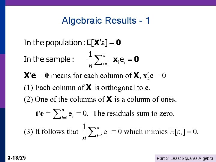
Algebraic Results - 1 3 -18/29 Part 3: Least Squares Algebra

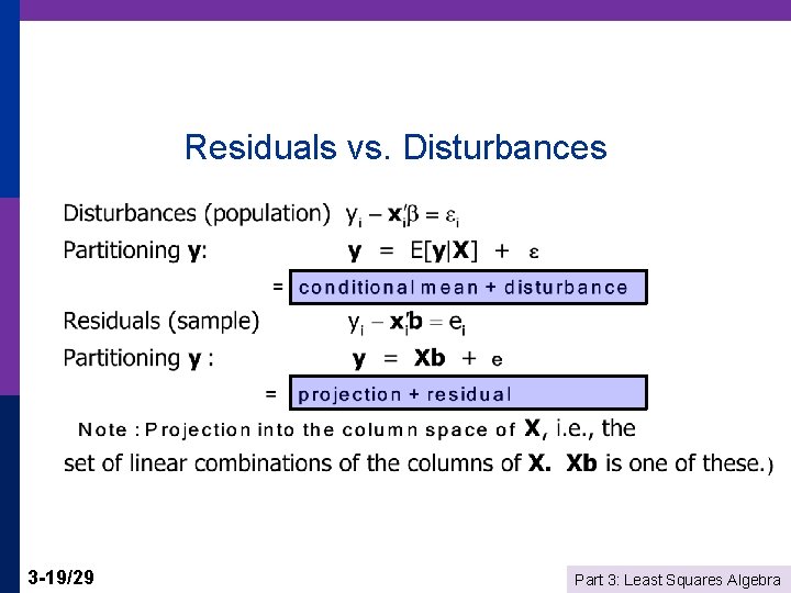
Residuals vs. Disturbances 3 -19/29 Part 3: Least Squares Algebra

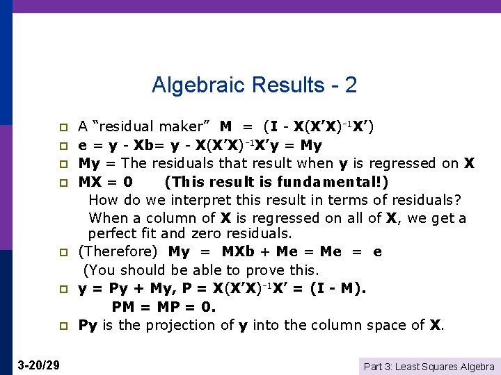
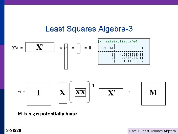
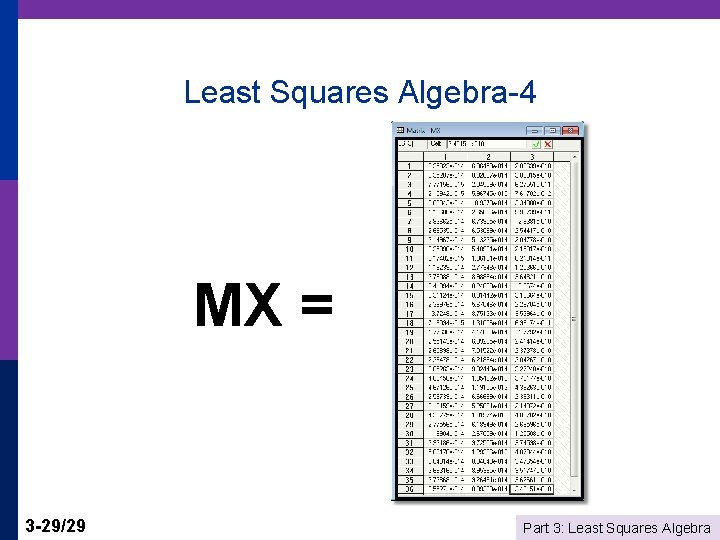
Algebraic Results - 2 p p p p 3 -20/29 A “residual maker” M = (I - X(X’X)-1 X’) e = y - Xb= y - X(X’X)-1 X’y = My My = The residuals that result when y is regressed on X MX = 0 (This result is fundamental!) How do we interpret this result in terms of residuals? When a column of X is regressed on all of X, we get a perfect fit and zero residuals. (Therefore) My = MXb + Me = e (You should be able to prove this. y = Py + My, P = X(X’X)-1 X’ = (I - M). PM = MP = 0. Py is the projection of y into the column space of X. Part 3: Least Squares Algebra

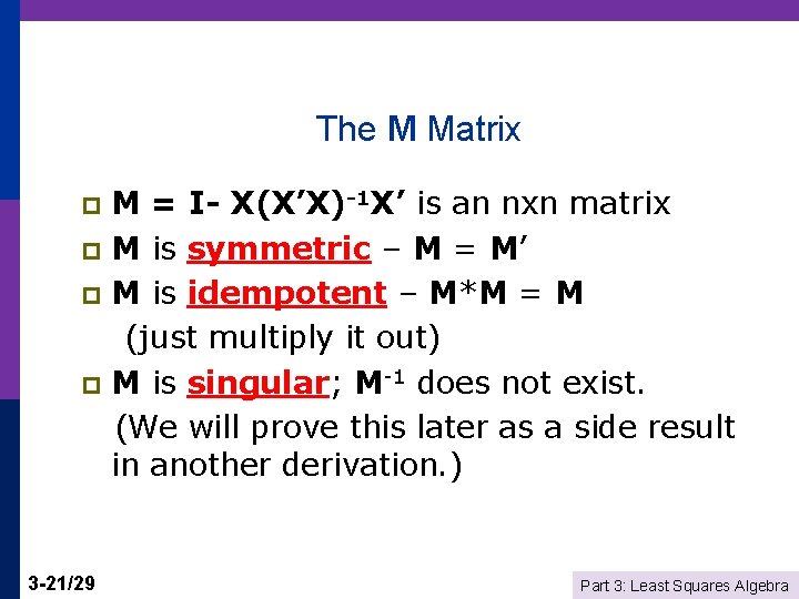
The M Matrix M = I- X(X’X)-1 X’ is an nxn matrix p M is symmetric – M = M’ p M is idempotent – M*M = M (just multiply it out) p M is singular; M-1 does not exist. (We will prove this later as a side result in another derivation. ) p 3 -21/29 Part 3: Least Squares Algebra

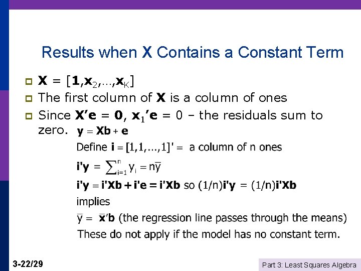
Results when X Contains a Constant Term p p p X = [1, x 2, …, x. K] The first column of X is a column of ones Since X’e = 0, x 1’e = 0 – the residuals sum to zero. 3 -22/29 Part 3: Least Squares Algebra

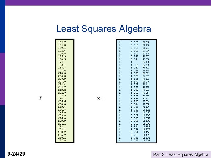
U. S. Gasoline Market, 1960 -1995 3 -23/29 Part 3: Least Squares Algebra

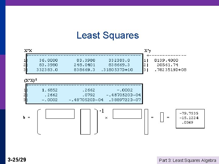
Least Squares Algebra 3 -24/29 Part 3: Least Squares Algebra

Least Squares 3 -25/29 Part 3: Least Squares Algebra

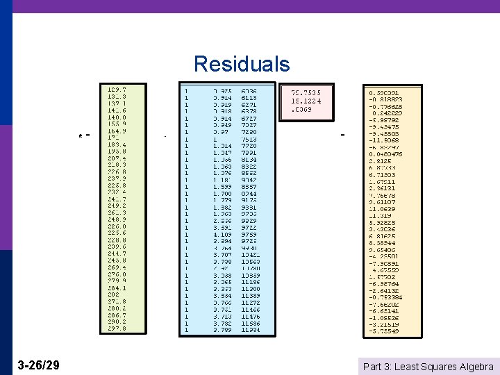
Residuals 3 -26/29 Part 3: Least Squares Algebra

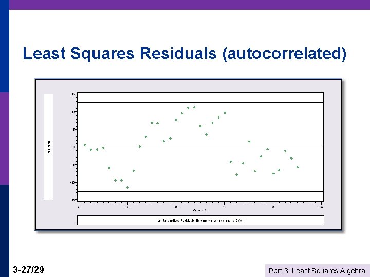
Least Squares Residuals (autocorrelated) 3 -27/29 Part 3: Least Squares Algebra

Least Squares Algebra-3 M is n n potentially huge 3 -28/29 Part 3: Least Squares Algebra

Least Squares Algebra-4 MX = 3 -29/29 Part 3: Least Squares Algebra