Regression Models Professor William Greene Stern School of

Regression Models Professor William Greene Stern School of Business IOMS Department of Economics 8 -1/35 Part 8: Regression Diagnostics

Regression and Forecasting Models Part 8 – Multicollinearity, Diagnostics 8 -2/35 Part 8: Regression Diagnostics

Multiple Regression Models p p Multicollinearity Variable Selection – Finding the “Right Regression” n p 8 -3/35 Stepwise regression Diagnostics and Data Preparation Part 8: Regression Diagnostics

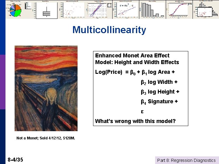
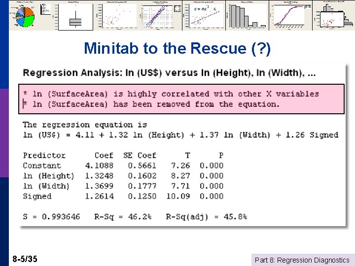
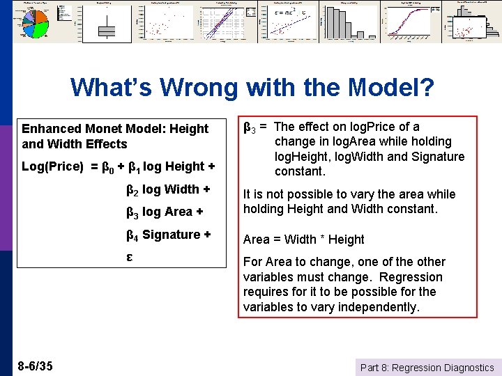
Multicollinearity Enhanced Monet Area Effect Model: Height and Width Effects Log(Price) = β 0 + β 1 log Area + β 2 log Width + β 3 log Height + β 4 Signature + ε What’s wrong with this model? Not a Monet; Sold 4/12/12, $120 M. 8 -4/35 Part 8: Regression Diagnostics

Minitab to the Rescue (? ) 8 -5/35 Part 8: Regression Diagnostics

What’s Wrong with the Model? Enhanced Monet Model: Height and Width Effects Log(Price) = β 0 + β 1 log Height + β 2 log Width + 8 -6/35 β 3 = The effect on log. Price of a change in log. Area while holding log. Height, log. Width and Signature constant. β 3 log Area + It is not possible to vary the area while holding Height and Width constant. β 4 Signature + Area = Width * Height ε For Area to change, one of the other variables must change. Regression requires for it to be possible for the variables to vary independently. Part 8: Regression Diagnostics

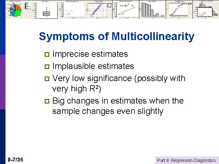
Symptoms of Multicollinearity Imprecise estimates p Implausible estimates p Very low significance (possibly with very high R 2) p Big changes in estimates when the sample changes even slightly p 8 -7/35 Part 8: Regression Diagnostics

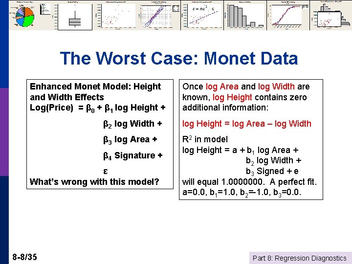
The Worst Case: Monet Data Enhanced Monet Model: Height and Width Effects Log(Price) = β 0 + β 1 log Height + β 2 log Width + log Height = log Area – log Width β 3 log Area + R 2 in model log Height = a + b 1 log Area + b 2 log Width + b 3 Signed + e will equal 1. 0000000. A perfect fit. a=0. 0, b 1=1. 0, b 2=-1. 0, b 3=0. 0. β 4 Signature + ε What’s wrong with this model? 8 -8/35 Once log Area and log Width are known, log Height contains zero additional information: Part 8: Regression Diagnostics

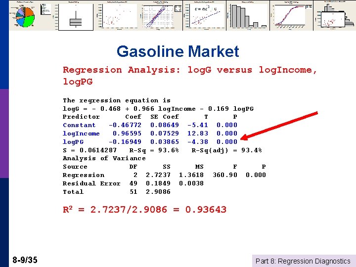
Gasoline Market Regression Analysis: log. G versus log. Income, log. PG The regression equation is log. G = - 0. 468 + 0. 966 log. Income - 0. 169 log. PG Predictor Coef SE Coef T P Constant -0. 46772 0. 08649 -5. 41 0. 000 log. Income 0. 96595 0. 07529 12. 83 0. 000 log. PG -0. 16949 0. 03865 -4. 38 0. 000 S = 0. 0614287 R-Sq = 93. 6% R-Sq(adj) = 93. 4% Analysis of Variance Source DF SS MS F P Regression 2 2. 7237 1. 3618 360. 90 0. 000 Residual Error 49 0. 1849 0. 0038 Total 51 2. 9086 R 2 = 2. 7237/2. 9086 = 0. 93643 8 -9/35 Part 8: Regression Diagnostics

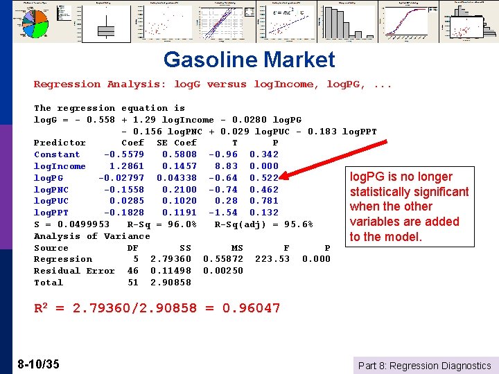
Gasoline Market Regression Analysis: log. G versus log. Income, log. PG, . . . The regression equation is log. G = - 0. 558 + 1. 29 log. Income - 0. 0280 log. PG - 0. 156 log. PNC + 0. 029 log. PUC - 0. 183 log. PPT Predictor Coef SE Coef T P Constant -0. 5579 0. 5808 -0. 96 0. 342 log. Income 1. 2861 0. 1457 8. 83 0. 000 log. PG -0. 02797 0. 04338 -0. 64 0. 522 log. PG is no longer log. PNC -0. 1558 0. 2100 -0. 74 0. 462 statistically significant log. PUC 0. 0285 0. 1020 0. 28 0. 781 when the other log. PPT -0. 1828 0. 1191 -1. 54 0. 132 variables are added S = 0. 0499953 R-Sq = 96. 0% R-Sq(adj) = 95. 6% Analysis of Variance to the model. Source DF SS MS F P Regression 5 2. 79360 0. 55872 223. 53 0. 000 Residual Error 46 0. 11498 0. 00250 Total 51 2. 90858 R 2 = 2. 79360/2. 90858 = 0. 96047 8 -10/35 Part 8: Regression Diagnostics

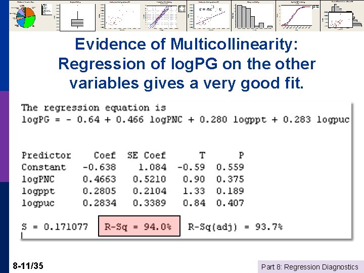
Evidence of Multicollinearity: Regression of log. PG on the other variables gives a very good fit. 8 -11/35 Part 8: Regression Diagnostics

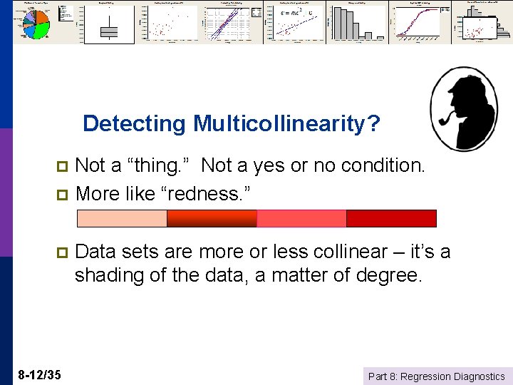
Detecting Multicollinearity? Not a “thing. ” Not a yes or no condition. p More like “redness. ” p p 8 -12/35 Data sets are more or less collinear – it’s a shading of the data, a matter of degree. Part 8: Regression Diagnostics

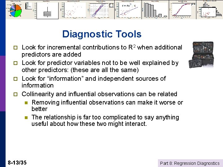
Diagnostic Tools p p Look for incremental contributions to R 2 when additional predictors are added Look for predictor variables not to be well explained by other predictors: (these are all the same) Look for “information” and independent sources of information Collinearity and influential observations can be related n Removing influential observations can make it worse or better n The relationship is far too complicated to say anything useful about how these two might interact. 8 -13/35 Part 8: Regression Diagnostics

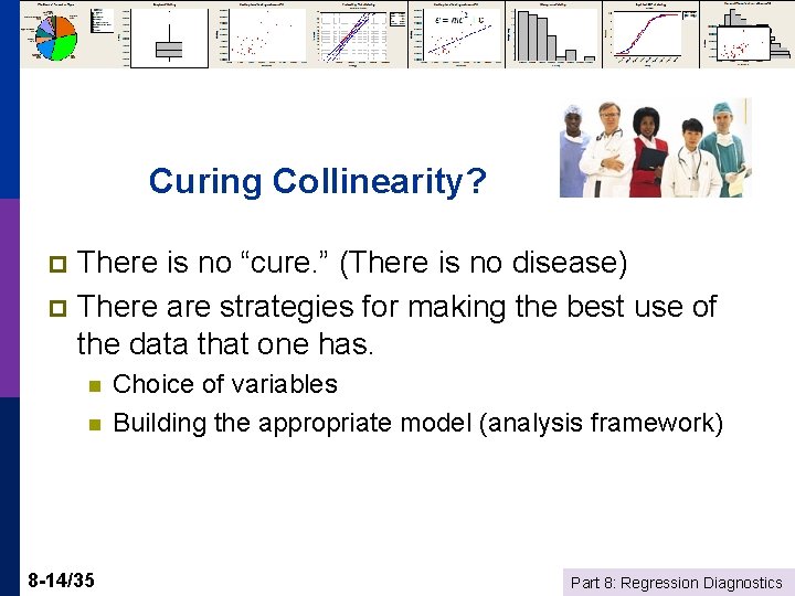
Curing Collinearity? There is no “cure. ” (There is no disease) p There are strategies for making the best use of the data that one has. p n n 8 -14/35 Choice of variables Building the appropriate model (analysis framework) Part 8: Regression Diagnostics

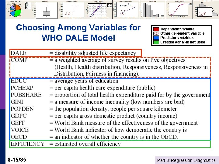
Choosing Among Variables for WHO DALE Model 8 -15/35 Dependent variable Other dependent variable Predictor variables Created variable not used Part 8: Regression Diagnostics

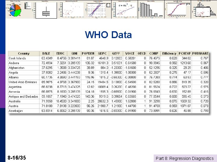
WHO Data 8 -16/35 Part 8: Regression Diagnostics

Choosing the Set of Variables p p Ideally: Dictated by theory Realistically n n n p Practically n n 8 -17/35 Uncertainty as to which variables Too many to form a reasonable model using all of them Multicollinearity is a possible problem Obtain a good fit Moderate number of predictors Reasonable precision of estimates Significance agrees with theory Part 8: Regression Diagnostics

Stepwise Regression p p p 8 -18/35 Start with (a) no model, or (b) the specific variables that are designated to be forced to into whatever model ultimately chosen (A: Forward) Add a variable: “Significant? ” Include the most “significant variable” not already included. (B: Backward) Are variables already included in the equation now adversely affected by collinearity? If any variables become “insignificant, ” now remove the least significant variable. Return to (A) This can cycle back and forth for a while. Usually not. Ultimately selects only variables that appear to be “significant” Part 8: Regression Diagnostics

Stepwise Regression Feature 8 -19/35 Part 8: Regression Diagnostics

Specify Predictors All predictors Subset of predictors that must appear in the final model chosen (optional) No need to change Methods or Options 8 -20/35 Part 8: Regression Diagnostics

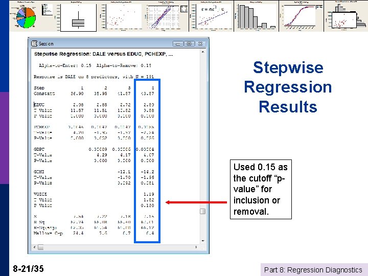
Stepwise Regression Results Used 0. 15 as the cutoff “pvalue” for inclusion or removal. 8 -21/35 Part 8: Regression Diagnostics

Stepwise Regression p What’s Right with It? n n n p What’s Wrong with It? n n 8 -22/35 Automatic – push button Simple to use. Not much thinking involved. Relates in some way to connection of the variables to each other – significance – not just R 2 No reason to assume that the resulting model will make any sense Test statistics are completely invalid and cannot be used for statistical inference. Part 8: Regression Diagnostics

Data Preparation p Get rid of observations with missing values. n Small numbers of missing values, delete observations n Large numbers of missing values – may need to give up on certain variables n There are theories and methods for filling missing values. (Advanced techniques. Usually not useful or appropriate for real world work. ) p Be sure that “missingness” is not directly related to the values of the dependent variable. E. g. , a regression that follows systematically removing “high” values of Y is likely to be biased if you then try to use the results to describe the entire population. 8 -23/35 Part 8: Regression Diagnostics

Using Logs p p 8 -24/35 Generally, use logs for “size” variables Use logs if you are seeking to estimate elasticities Use logs if your data span a very large range of values and the independent variables do not (a modeling issue – some art mixed in with the science). If the data contain 0 s or negative values then logs will be inappropriate for the study – do not use ad hoc fixes like adding something to y so it will be positive. Part 8: Regression Diagnostics

More on Using Logs 8 -25/35 p Generally only for continuous variables like income or variables that are essentially continuous. p Not for discrete variables like binary variables or qualititative variables (e. g. , stress level = 1, 2, 3, 4, 5) p Generally be consistent in the equation – don’t mix logs and levels. p Generally DO NOT take the log of “time” (t) in a model with a time trend. TIME is discrete and not a “measure. ” Part 8: Regression Diagnostics

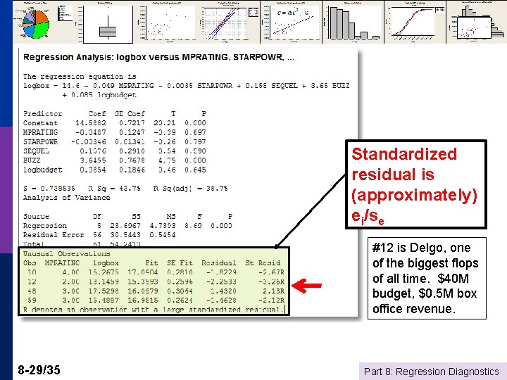
Residuals p p Residual = the difference between the actual value of y and the value predicted by the regression. E. g. , Switzerland: n n n p 8 -26/35 Estimated equation is DALE = 36. 900 + 2. 9787*EDUC +. 004601*PCHexp Swiss values are EDUC=9. 418360, PCHexp=2646. 442 Regression prediction = 77. 1307 Actual Swiss DALE = 72. 71622 Residual = 72. 71622 – 77. 1307 = -4. 41448 The regresion “overpredicts” Switzerland Part 8: Regression Diagnostics

Using Residuals As indicators of “bad” data p As indicators of observations that deserve attention p As a diagnostic tool to evaluate the regression model p 8 -27/35 Part 8: Regression Diagnostics

When to Remove “Outliers” Outliers have very large residuals p Only if it is ABSOLUTELY necessary p n n p 8 -28/35 The data are obviously miscoded There is something clearly wrong with the observation Do not remove outliers just because Minitab flags them. This is not sufficient reason. Part 8: Regression Diagnostics

Standardized residual is (approximately) ei/se #12 is Delgo, one of the biggest flops of all time. $40 M budget, $0. 5 M box office revenue. 8 -29/35 Part 8: Regression Diagnostics

Units of Measurement y = b 0 + b 1 x 1 + b 2 x 2 + e p If you multiply every observation of variable x by the same constant, c, then the regression coefficient will be divided by c. p E. g. , multiply X by. 001 to change $ to thousands of $, then b is multiplied by 1000. b times x will be unchanged. p 8 -30/35 Part 8: Regression Diagnostics

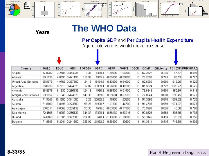
Scaling the Data Units of measurement and coefficients p Macro data and per capita figures p n n p Micro data and normalizations n 8 -31/35 Gasoline data WHO data R&D and Profits Part 8: Regression Diagnostics

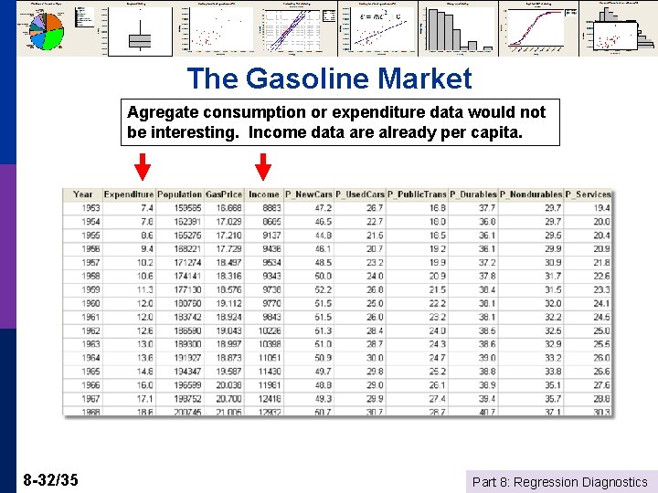
The Gasoline Market Agregate consumption or expenditure data would not be interesting. Income data are already per capita. 8 -32/35 Part 8: Regression Diagnostics

Years The WHO Data Per Capita GDP and Per Capita Health Expenditure. Aggregate values would make no sense. 8 -33/35 Part 8: Regression Diagnostics

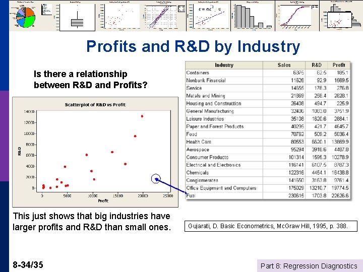
Profits and R&D by Industry Is there a relationship between R&D and Profits? This just shows that big industries have larger profits and R&D than small ones. 8 -34/35 Gujarati, D. Basic Econometrics, Mc. Graw Hill, 1995, p. 388. Part 8: Regression Diagnostics

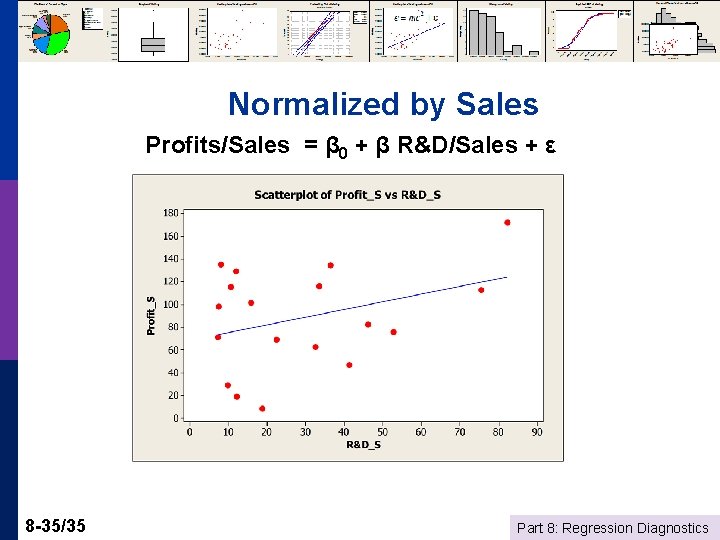
Normalized by Sales Profits/Sales = β 0 + β R&D/Sales + ε 8 -35/35 Part 8: Regression Diagnostics